Danish Meteorological Institute, Lyngbyvej 100,DK-2100 . Email: boc@dmi.dk
FIGURES
Abstract
Downward propagation of anomalies in the Northern Hemisphere winter is presented in a hierarchy of models and compared to the NCEP reanalysis. The models inlcude simplistic models and GCMs in perpetual January mode and with the annual cycle included. We focus the study on intraannual timescales between 30 and 350 days.
All models show downward propagation on realistic timescales although the structure and amplitude differ. With increasing complexity of the models the resemblance to the NCEP reanalysis grows.
In the models including the troposphere and in the reanalysis the downward propagation and the Arctic oscillation are connected: When positive anomalies reach the surface the phase of the Arctic Oscillation tends to be positive.
The vacillations are driven by large scale waves which penetrate
from the troposphere into the stratosphere, where they break and
drive the zonal mean circulation. The downward propagation is
a consequence of the fact that the mean flow itself determines
the vertical extent of the propagation of the planetary waves.
A minimal model based on these principles is formulated.
Introduction
The understanding of the link between the troposphere and stratosphere has increased with the discovery (Thompson and Wallace, 1998) of a deep vertical coupling connected to the annular, circumpolar mode known as the Arcrtic oscillation. Furthermore, the downward propagation from the stratosphere to the troposphere found in both data (Baldwin and Dunkerton, 1999) and model (Christiansen, 2000) has raised the question as to what extent the stratosphere is controlling the troposphere.
This brief contribution will demonstrate the existence of downward propagation in simplistic as well as comprehensive models. Even simple models without a troposphere will show downward propagation in the form of stratopsheric vacillations (see also Holton and Mass, 1976; Christiansen ,1999, Scaife and James, 2000, Kodera and Kuroda, 2000). In the general circulation model experiments the structure and timescale of the downward propagation are in exellent agreement with the NCEP reanalysis.
Analysing the GCM experiments and the NCEP reanalysis shows that the downward propagation is driven by the vertical component of the Eliassen-Palm flux. A minimal model is constructed according to this idea.
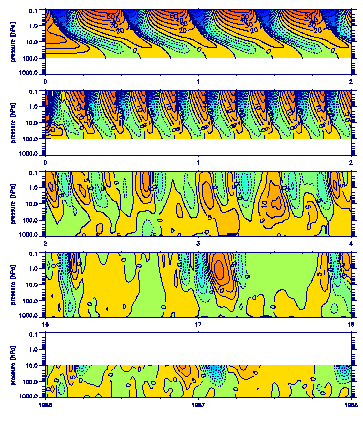
Figure 1 The downward propagation in the northern hemisphere (60 N) for a series of models of increasing complexity and for the NCEP reanalysis (bottom). Zonal mean zonal wind anomalies are shown as function of pressure and time (years). The first panel is the minimal model defined below, the second panel is the Holton-Mass model, the third panel the ARPEGE GCM in perpetual January mode, the fourth panel is the ARPEGE GCM with the annual cycle included, and the bottom panel is the NCEP reanalysis. Data have been band-passed filtered to include only timescales between 30 and 350 days.
Downward propagation
Downward propagation of zonal mean zonal wind anomalies is found in a hierarchy of models as well as in the NCEP reanalysis. Figure 1 shows zonal mean zonal wind anomalies as function of height and time for a minimal model (see below), the Holton-Mass model, a perpetual January GCM experiment, a GCM experiment with the annual cycle, and the NCEP reanalysis. For the GCM experiment and the reanalysis 60N is selected. For the simplistic models the parameters are chosen to represent northern hemisphere winter.
The downward propagation is obvious in all the plots. In the simplistic models the vacillations have a regular recurrence: the termination of one event near the lower boundary is followed by the birth of a new event near the top of the model. In the GCM the vacillations are more irregular, in particular when the annual cycle is included. In both the GCM including the annual cycle and in the reanalysis very little variability is seen in the half-year from May to October. In the half-year from November to April the variability is considerable. All winter half-years show at least one event of each sign while a few show two or more such events. In both GCM and reanalysis the events often reach the surface.
The average properties of the downward propagation in the GCM with the annual cycle and the reanalysis are captured in Fig. 2 which shows the lagged correlations between the zonal mean zonal wind at 60 N ,10 hPa and the zonal mean zonal wind at all other levels at 60 N. Correlations significant on the four sigma level reach the surface in both model and reanalysis and the time of propagation from 10 hPa to the surface is about 15 days. In the model it takes additional 10 days for the events to propagate from 0.1 hPa to 10 hPa.
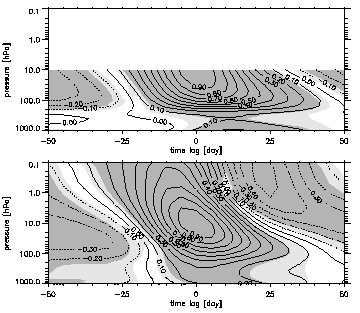
Figure 2 Correlations of the zonal mean zonal wind at 60 N with that at 10 hPa as function of pressure and time-lag. The upper and lower panel shows the NCEP reanalysis and the model, respectively. Light and dark shading identify regions where the correlations are significantly different from zero on two sigma and four sigma levels.
Connection to the troposphere
Figures 3 and 4 compare the GCM with the annual cycle to the NCEP reanalysis. A Principal Component Analysis has been performed of the sea-level pressure in the model and the reanalysis. The region north of 20 N is included and the data are weighted with the square root of the area they represent. The resulting leading EOFs (Fig. 4) are very similar and display the now familiar signature of the Arctic Oscillation: a dominantly annual, circumpolar structure with the node around 60 N and maxima over the Atlantic and Pacific oceans. In the model the two maxima have approximately the same strength while the Atlantic center is strongest in the reanalysis. Both model and reanalysis agree on the weakness of the pattern over the central part of the Eurasian continent and the displacement of the negative polar center towards the North Atlantic region. The leading EOFs in the model and reanalysis explain 14 and 23 % of the total variance.
Figure 3 shows the correlations between the first principal component of the surface pressure and the zonal mean zonal winds in the meridional plane. Below 10 hPa both model and reanalysis display the dipole structure known from other studies with the cross-over between negative and positive correlations near 45 N. In the model the correlations change sign above 3-4 hPa north of 45 N and above 10-20 hPa south of 45 due to the downward propagation of anomalies: when positive anomalies reach the surface negative anomalies dominate the upper stratosphere.
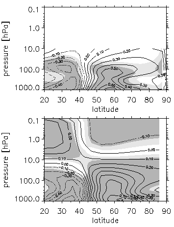
Figure 3 Correlations between the zonal mean zonal wind and the first principal component of the surface pressure. Top panel is the reanalysis and lower panel is the model.
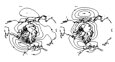
Figure 4 The leading EOF of the surface pressure in the reanalysis (left) and the model (right). These modes explain 14 and 19% of the total variance. The scaling is arbitrary.
The wave forcing
To further study the relations between the eddy flux and the vacillations
we now present lagged cross covariances between the zonal mean
zonal wind and the terms in the zonal momentum balance equation,
i.e., the zonal mean wind tendency $\partial \overline{u}/ \partial
t$, the Coriolis term $f \overline{v}^{*}$, and the two components
of the eddy forcing![]()
We chose the zonal mean zonal wind at 10 hPa and concentrate
as before on 60 N. The covariances with the tendency (fFig 5,
top) are easily understood: at 10 hPa large (small) values of
the zonal wind have been preceded by acceleration (deceleration)
and are followed by deceleration (acceleration). The vertical
tilt in cross-over between positive and negative covariances is
an effect of the downward propagation.
The strong similarity between the first and last panel in Fig. 5 shows that the downward propagation is driven by wave mean interactions related to the waves resolved in the reanalysis. We also note that the vertical wave flux dominates and that the horizontal wave flux only plays a minor role in the stratosphere.
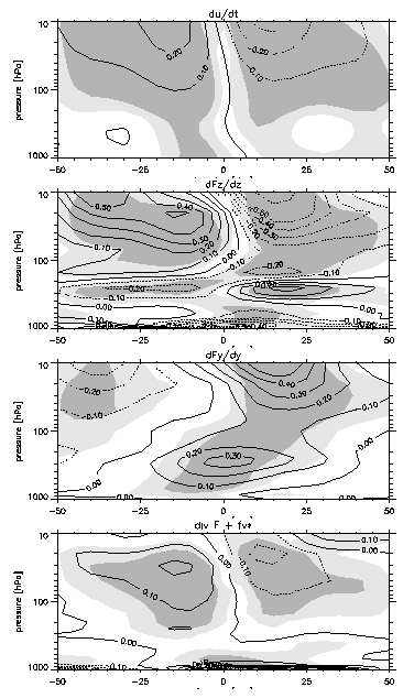
Figure 5 Covariance between the zonal mean wind at 10 hPa, 60 N and the terms in the balance equation for zonal momentum as function of lag (days) and pressure. Shading as in Fig. 2.
A minimal model
The minimal model captures the basic physics of the vacillations
and llustrates the basic principles behind the downward propagation:
the competition between wave-driving and the radiative damping.
It is in agreement with the conclusion from Fig. 5 that the vertical
wave flux dominates. Stripping the transformed Eulerian-mean equation
to its back-bone results in:
![]()
The zonal acceleration is given by a relaxation towards ur and by the wave forcing ![]() . In addition we have put in a diffusion term partly to account
for the non-localness of the original equation.
. In addition we have put in a diffusion term partly to account
for the non-localness of the original equation.
The Eliassen-Palm flux represents the propagation of eddy activity.
In the optical limit the vertical propagation of F is given by
![]()
where F0 is the wave forcing at the lower boundary, z=0, taken as the
tropopause. The resistance g depends on the mean flow u and diverge when u gets close to the group velocity c of the waves. The exact functional
form depends on the wave type. Here we take
![]()
The system resembles the model of the quasi-biennial oscillation studied by Plumb (1977), which is driven by two waves at the lower boundary and which does not include the relaxation. In the present work only one wave is needed. As the Holton-Mass model (Holton and Mass, 1976) this minimal model undergoes a Hopf-bifurcation from a quiescent state to an oscillating state when the forcing at the lower boundary is increased above a threshold value. The Hopf-bifurcation has also been identified in the GCM (Christiansen, 1999).
Conclusion
The fact that the downward propagation is so well captured by even the simplest models allows us to believe that such models will be able to provide an answer to the question of how strongly changes in the stratosphere will be felt near the surface. Changes in the stratosphere take place due to the depletion of stratospheric ozone and the increasing levels of carbon-dioxide. However, also changes in the stratopsheric structure related to the 11-year solar cycle are often reported. On shorter timescales understanding of the downward propagation may improve weather and seasonal forecasts.
References
Baldwin M. P., and T. J. Dunkerton, Propagation of the Arctic Oscillation from the stratosphere to the troposphere, J. Geophys. Res., 104, 30937-30946, 1999.
Christiansen, B., Stratospheric vacillations in a general circulation model, J. Atmos. Sci., 56, 1858-1872, 1999.
Christiansen, B., A model study of the dynamical connection between the Arctic Oscillation and stratospheric vacillations, to appear in J. Geophys. Res., 2000.
Holton, J. R., and C. Mass, Stratospheric vacillation cycles, J. Atmos. Sci., 33, 2218-2225, 1976.
Kodera K., and Y. Kuroda, A mechanistic model study of slowly
propagating
coupled stratosphere-troposphere variability, J. Geophys. Res., 105,12,361-12,370, 2000.
Plumb, R. A., The interaction of two internal waves with the mean flow: Implications for the theory of the quasi-biennial oscillation, J. Atmos. Sci., 34, 1847-1858., 1977.
Scaife, A. A., and I. N. James, Response of the stratosphere to interannual variability of tropospheric planetary waves, Q. J. R. Meteorol. Soc., 126, 275-297, 2000.
Thompson D. W. J, and J. M. Wallace, The Arctic Oscillation signature in the wintertime geopotential height and temperature fields, Geophys. Res. Lett., 25, 1297-1300, 1998.
Back to
| Session 1 : Stratospheric Processes and their Role in Climate | Session 2 : Stratospheric Indicators of Climate Change |
| Session 3 : Modelling and Diagnosis of Stratospheric Effects on Climate | Session 4 : UV Observations and Modelling |
| AuthorData | |
| Home Page | |