Previous: Preliminary analysis Next: Conclusions Up: Ext. Abst.
Interannual variability study
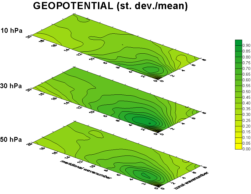
Based on the monthly values of all spectral coefficients obtained from the reanalyses of Free University in Berlin we tested the variability of the data by means of normalized standard deviations of the coefficients, both for geopotential and temperature. It is plotted in Fig. 11 and Fig. 12, respectively, as a ratio of the standard deviation and the mean for all data from available levels. The high variability can be seen just for low significant wavenumbers, in accordance with the main principles and objections of the method. We also present on similar figures for geopotential the sensitivity of the spherical harmonics components to quasi-biennial oscillations for 30 and 50 hPa levels by means of the ratio between the values for westerly and easterly phase of QBO (see Fig. 13) as well as for variability of these phases by means of the ratio of standard deviations (see Fig. 14).

Figure 11. The variability of the data of FUB by means of normalized standard deviations of the coefficients for geopotential.
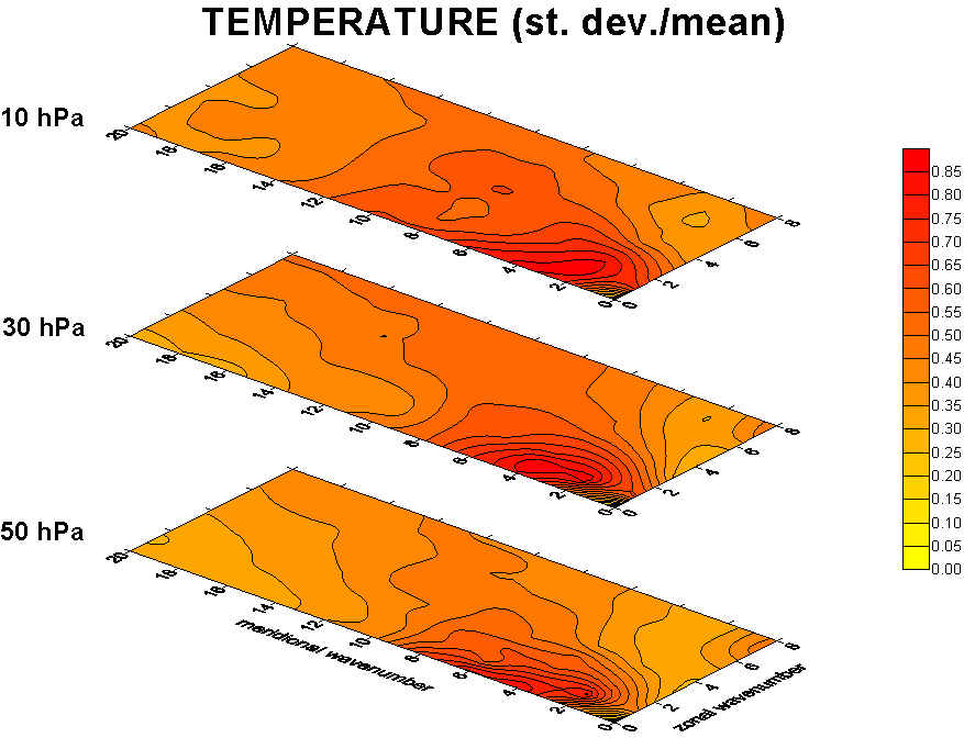
Figure 12. The variability of the data of FUB by means of normalized standard deviations of the coefficients for temperature.
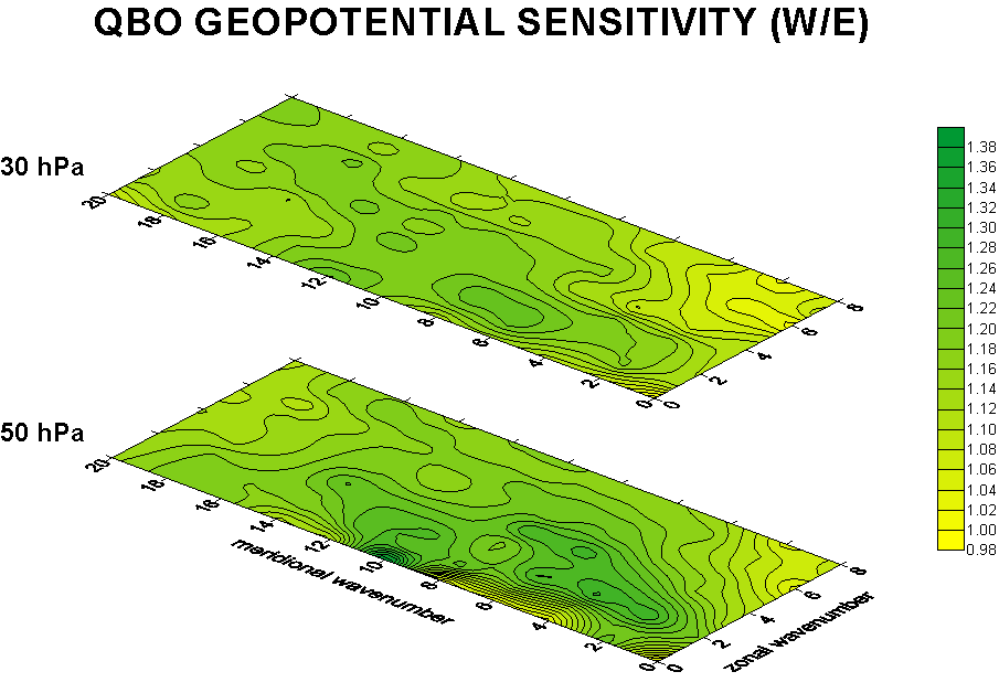
Figure 13. The sensitivity of the data of FUB for westerly and easterly phase of QBO for geopotential.
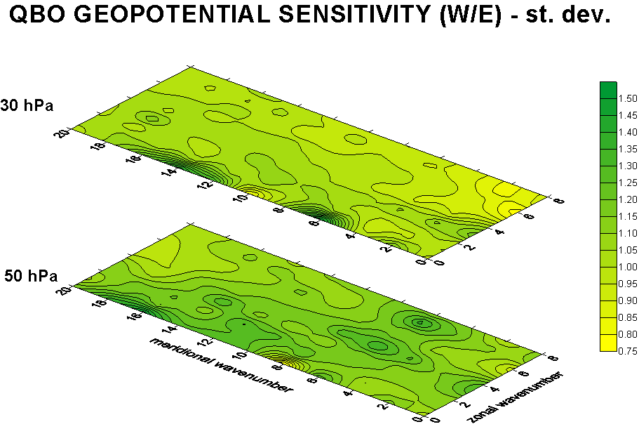
Figure 14. The sensitivity of the data of FUB for variability during the westerly and easterly phase of QBO for geopotential .
Based on the monthly values of some spectral coefficients we analyzed the interannual variability with respect to other available factors as well. We have used both extraterrestrial characteristics and the parameters developed from long-term atmospheric observations. Solar activity in terms of the F10.7 index was available from the National Goddard Data Center, as well as geomagnetic activity data in terms of the AP index. The latter group of factors was created by ENSO ö standardized monthly values of the Southern Oscillations index ö and QBO characteristics mentioned previously based on standardized monthly Singapore winds at the 30 and 50 hPa levels. Some comparisons, using cross-correlation analysis for geopotential wave number 5-1, are shown in Fig. 15 for solar activity and in Fig. 16 for geomagnetic activity. This served mainly to find some similarities between some coefficients and indices and to estimate the time scale of the potential response of the spectral coefficients to the individual parameters. To avoid the periodicity of the annual cycle, we worked with moving averages with a 12-month span which makes sense mainly for the spectral coefficients, for the series of extraterrestrial indices it yields better results due to lower dispersion. In the further analysis of the regression relations, we have used shifted series regarding the causality of the potential influence, i.e., extraterrestrial parameters as lagged independent variables unlike the other "circulation parameters" like ENSO or QBO, where the "causality" does not seem to have the physical meanings and only criterion of the better correlation may be accepted.
Figure 15. Cross-correlations analysis of geopotential component of wave number 5-1 against solar activity parameter (F10.7) with lag in months.
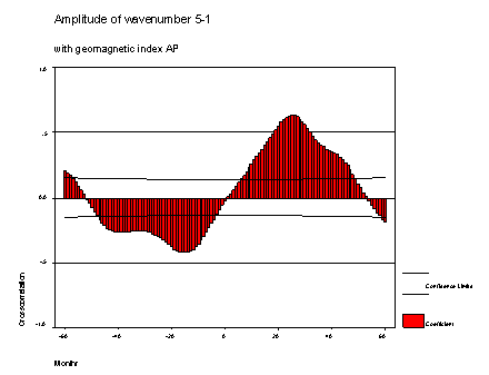
Figure 16. Cross-correlations analysis of geopotential component of wave number 5-1 against geomagnetic activity index (AP) with lag in months.
We have run numerous experiments with the linear regression model with the significant geopotential and temperature components used as dependent variables, series of extraterrestrial indices and other circulation parameters with the appropriate shifts being independent variables. In some cases it seems to be convenient to test the influence of appropriate temperature component in geopotential regression and vice versa. We have obtained quite good results for some of them although for other wave numbers it seems to be impossible to find any reliable connections. Anyway, the method of the spectral decomposition appears to be useful seeking possible effects in global scale. The systematic analysis will be a subject of further studies, here we will limit ourselves to present quite interesting results of the experiment with the component of wave number 5-1, which corresponds to four trough shape of polar vortex and which manifests very strong dependence.
Table 1 describes the first attempt to estimate parameters of the linear regression model with solar and geomagnetic activity as the only independent variables. It can be seen quite high correlation of such a model with the smoothed data. It is evident the dominant influence of solar activity comparing to geomagnetic activity, which can be confirmed also in Tab. 2, where temperature component of wave number 5-1 is included as well. It should be mentioned that temperature actually is not independent variable with regard to the geopotential and, moreover, our temperature record in data is not complete in 1992, but solar activity still remains the dominant factor of our regression analysis. The results of these experiments are presented in Fig. 17 and Fig. 18 for both modifications of the model, together with standardized residua comparison (see Fig. 19). It should be mentioned here that other circulation parameters do not help to fit better our model to the data, although it seems that some strong events of ENSO could result in higher departures, as well as, e.g., stratospheric warmings. Moreover, concerning the QBO, we have tested the model for QBO positive and negative, i.e., west and east phases, respectively. The results are even better for the first case, the similar model gives correlation 0.967.
Table 1. Linear regression model results for geopotential component of wave number 5-1 (Z51 smoothed by moving average ö MA with 12 months span) against solar activity (represented by F10.7 index also smoothed ö F10.7_1 and lagged by 45 months) and geomagnetic activity (represented by AP index also smoothed ö AP_1 and lagged by 42 months).
Model Summary
|
|
|
|
|
|
|
|
|
|
|
|
|
|
|
Coefficients
|
|
|
|
|
|
|
|
|
|
|
|
|
|
|
|
|
|
|
|
|
|
|
|
|
|
|
|
|
|
|
|
|
|
|
a Predictors: (Constant), LAGS(F10.7_1,45)
b Predictors: (Constant), LAGS(F10.7_1,45), LAGS(AP_1,42)
Dependent Variable: MA(Z51,12,12)
Table 2. Linear regression model results for geopotential component of wave number 5-1 (Z51) against solar activity (represented by F10.7 measurement), geomagnetic activity (represented by AP index) ö similarly as in Tab.1. and temperature component of wave number 5-1 (TZ51 also smoothed by moving average ö MA with 12 months span).
Model Summary
|
|
|
|
|
|
|
|
|
|
|
|
|
|
|
|
|
|
|
|
Coefficients
|
|
|
|
|
|
|
|
|
|
|
|
|
|
|
|
|
|
|
|
|
|
|
|
|
|
|
|
|
|
|
|
|
|
|
|
|
|
|
|
|
|
|
|
|
|
|
|
|
|
|
|
|
|
|
|
|
|
|
a Predictors: (Constant), LAGS(F10.7_1,45)
b Predictors: (Constant), LAGS(F10.7_1,45), MA(TZ51,12,12)
c Predictors: (Constant), LAGS(F10.7_1,45), MA(TZ51,12,12), LAGS(AP_1,42)
Dependent Variable: MA(Z51,12,12)
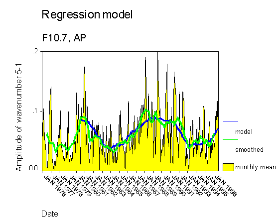
Figure 17. Linear regression analysis of the geopotential height of 30hPa level, spectral component with wave number 5-1.
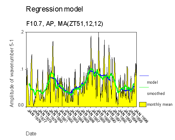
Figure 18. Linear regression analysis of the geopotential height of 30hPa level, spectral component with wave number 5-1, improvement by inclusion of appropriate temperature component.
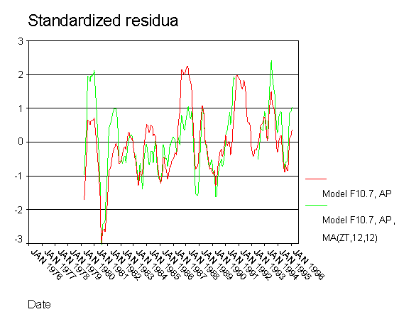
Figure 19. Linear regression analysis of the geopotential height of 30hPa level, spectral component with wave number 5-1, plots of residuals for both the models.