Southern Hemisphere ozone behavior during 1994 austral winter  

• Introduction
• Data 
• Mean Fields
• Case Study
• Conclusions
• Acknowledgements
• References

FIGURES

• Figures 1a, 1b
• Figure 2
• Figure 3
• Figure 4
• Figure 5
• Figure 6
• Figures 7a, 7b
• Figure 8

1. Introduction

Since long ago it has been recognised the relationship between ozone and atmospheric fields from scales ranging from decadal to interdiurnal. While for the long time-scales ozone is influenced by the atmosphere and viceversa, from a couple of weeks to days, ozone variability is mainly attributed to dynamical effects, as the ozone mixing ratio is a quasi-conserved tracer in the lower-stratosphere (Andrews et al. 1987). As a consequence, a clear correspondence between areas of maximum synoptic activity and regions of large ozone fluctuations is established. The nature of such correspondence may be understood in terms of baroclinic waves producing horizontal and vertical motions that affect the ozone distribution, as ozone partial pressure is  maximum in the lower-stratosphere, near the tropopause where this waves also attain a maximum (Vigliarolo et al. 2000 and references therein). Therefore, it is of interest to investigate in detail such dynamical-ozone changes for particular cases. In this paper an extreme ozone event is studied over southern South America (hereafter SA), a region that reports minimum winter mean ozone content and moderate to high ozone daily-variability (Vigliarolo et al. 2000).

2. Data 

The dataset is based on 1994 July NCEP four-daily reanalyses of standard meteorological variables given in constant pressure levels ranging from surface to 10-hPa and also over isentropic surfaces in the upper troposphere and lower stratosphere. From 100 to 10-hPa, the vertical velocity field was estimated using the thermodynamic equation under adiabatic conditions. Total ozone data from Meteor 3/Toms (version 7) was also used for the period of study, along with ozone mixing ratio profiles from SBUV/2 NOAA-11 (version 6; for reference see ftp://toms.gsfc.nasa.gov/pub/sbuv/sbuv2/readme.v612 ).

3. Mean Fields

3.a Stationary Waves

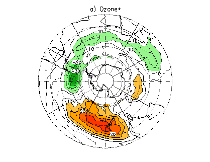
In this section the basic structure of stationary waves is discussed. Figure 1a shows ozone stationary component, calculated as the difference between July 1994 mean field and the corresponding zonal mean (denoted by "*"). South of 50ºS, ozone field depicts the typical wave number 1 that characterises the winter season, as described by Vigliarolo et al. (2000). Nevertheless, some differences could be appreciated. The high latitude-strong negative center is located slightly to the west and north regarding its climatological position and with values that are about two times greater. On the other hand, the positive center near 50ºS, 115ºW is much weaker (about 0.5 times) compared to climatology. Vigliarolo et al. (2000) have suggested that winter ozone stationary pattern over middle and high latitudes of Southern Hemisphere (SH) depends critically on the three dimensional structure of atmospheric stationary waves, which in turn produce ozone anomalies via both horizontal and vertical transports (although they also caution about the main role of non-conservative processes in contributing to ozone pattern).

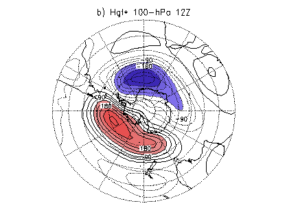
Figure 1: Zonal asymmetries of July 1994 mean fields for a) ozone and b) 100-hPa geopotential height. The contour interval is (a) 5 DU and (b) 50 m and the zero contour has been omitted.

The geopotential-height stationary wave at 100-hPa (fig.1b) also shows a wave number 1 structure over middle to high latitudes. But, although the location of the geopotential centers roughly coincides with the winter mean position (see Vigliarolo et al.2000, its fig.2b), the corresponding extremes for this particular July are more intense (about 1.8 times) and displaced towards southern SA. In agreement, a westward displacement of the maximum of the subpolar jet from the Indian Ocean to 45ºS, 15ºW and a jet weakening along the high latitudes of Pacific Ocean are observed.

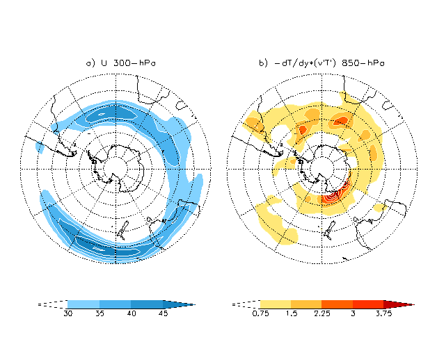
Figure 2: (a) 300-hPa mean zonal wind (contour interval 5ms^-1; only values above 30 ms^-1 are shown) and (b) mean  at 850-hPa (contour interval 0.75*10⁴ ºK² s^-1).

At middle latitudes of both southeastern Pacific and Indian oceans, ozone stationary pattern is related to geopotential height via the "tropopause effect" (Vigliarolo et al. 2000 and references therein). Moreover, a nearly continuous band of negative ozone anomalies centered along 40ºS extends from the Atlantic to the Central Indian Ocean and is related to geopotential positive anomalies by the same location; in the Pacific sector, relatively high positive ozone values are found in connection with a negative geopotential height center near New Zealand (figs.1a,b).

3.b Transients

The standard deviation of submonthly perturbations (constructed as the daily departures from July 1994 time mean) was chosen to represent transient wave activity. Ozone perturbation standard deviation (fig.3a) shows large values along the 40º-55ºS-latitude band, that roughly coincides with maximum 300-hPa geopotential height perturbation standard deviation maximums (fig.3b), thus confirming the main role of transients on driving ozone variability (Salby and Callahan 1993). In addition, the high-variability ozone centers are located poleward and maximize downstream with respect to the geopotential-height ones (Vigliarolo et al. 2000). Over southern SA, ozone perturbation standard deviation attains a maximum well above the mean winter standard deviation values for the region, that is in close association with a maximum of the geopotential-height standard deviation located over the same area (fig.3). In agreement, a minimum of ozone over this region of maximum submonthly wave activity is observed (fig.1a) that persisted throughout the month in association with a quasi-stationary, equivalent barotropic ridge centered at 55ºS, 90ºW (Figs.not shown).

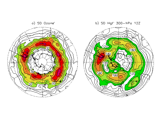
Figure 3: Standard deviation of daily departures from July 1994 time mean of: a) ozone (contour interval 5 DU) and b) 300-hPa geopotential height (contour interval 30 m).

Berbery and Vera (1996) have shown that during austral winter, low level baroclinicity attains its maximum over the subpolar jet latitudes with the highest values located between 30º and 60ºE.  The term (where the overbar denotes time mean and (') is the daily departure from time means, T is temperature and v is the meridional wind) is proportional to the mean baroclinic conversion and is shown for the 20º-65º latitude band at 850 hPa (fig.2b). Note that values south of this boundary are not plotted as it is difficult to assess the quality of the data around and over Antarctica, where both a combination of high terrain and steep slopes is found (Berbery and Vera 1996). In general this field show maximums located further west than the climatology. In particular, the displacement submonthly scale enhanced activity (fig. 3b) from its climatological position over the Indian Ocean to the central Atlantic Ocean seems to be associated with a conspicuous center of high baroclinicity near 55ºS, 25ºW that extends towards the Antarctica Peninsula (fig.2b). It is worth to point out that baroclinic conversion is not increased over southern SA, implying that other dynamical processes not considered here may account for the transient activity intensification over that region.

4. Case Study

4.a Synoptic Evolution

During the second week of the month, strong ozone perturbations were detected over southern SA, consisting of a transient ozone wave evolving with a southwest-northeast direction across the continent. From July 7^th to10^th (figs.4a-d) ozone values as low as 240 DU could be followed along four days from southern Patagonia to southwestern Atlantic. At the same time, high ozone values (up to 400 DU -fig.4b-) were observed to evolve over Buenos Aires and to the east.

The analogous evolution of the atmospheric fields shows a clear correspondence between ozone relative minimum (maximum) and: ridges (troughs), lowered (enhanced) tropopause pressure values (figs. 4e-h) and relative maximum (minimum) of potential vorticity on isentropic surfaces (figs. 4i-l). By use of a simple conceptual model, Vigliarolo et al. (2000) exhibited the dynamical relationship between a synoptic wave and the resulting ozone distribution, provided ozone-mixing ratio is conserved on these time scales. Moreover they showed by composite analysis for the preferred winter synoptic-scale mode of variability, that waves evolving along subpolar jet latitudes are responsible for the corresponding transient ozone-pattern. This is due to the barotropic-equivalent structure of these waves and the fact that ozone partial-pressure attains a maximum very close to the level where these waves also maximise.

In order to address the relative dynamical contributions of the atmospheric waves to ozone changes over southern SA region, two approaches are followed. The first, relates ozone daily changes to horizontal and vertical transports of ozone mixing ratio by transient motions (subsection 4b), while in the second ozone distribution is fitted to a multivariate linear relationship with tropopause pressure and potential vorticity at several isentropic levels (subsection 4c).

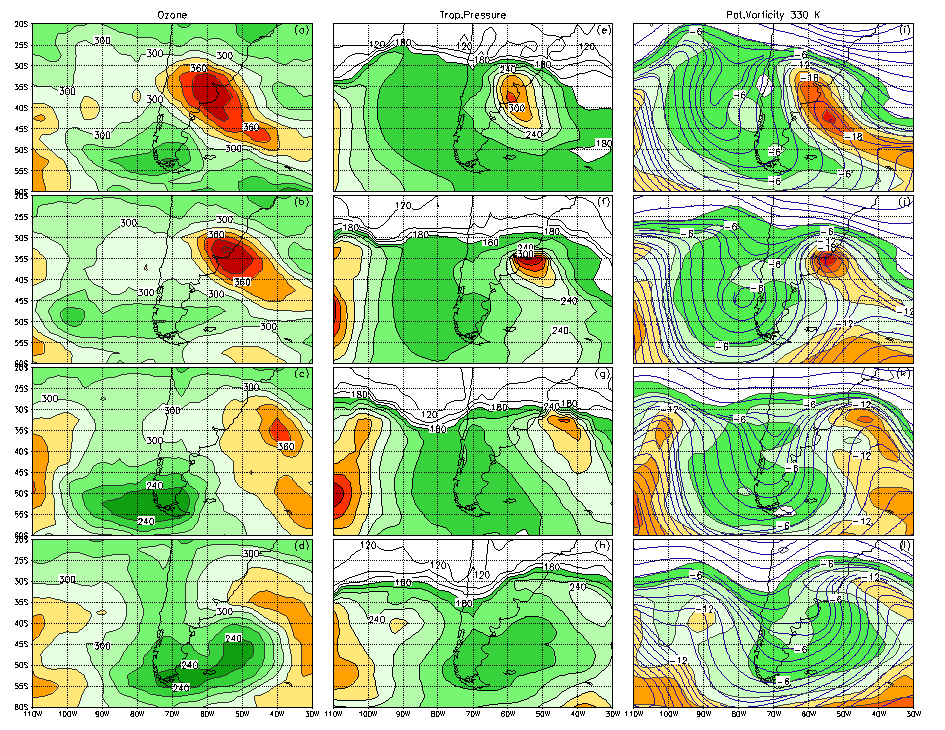
Figure 4: Temporal evolution from July 7^th to 10^th of: (a)-(d) ozone, (e)-(h) tropopause pressure, (i)-(l) potential vorticity (shaded) and streamlines (thick contours) on the 330ºK surface. Contour interval is (a)-(d) 20 DU; (e)-(h) 20 hPa; and (i)-(j) 2*10^-8 m2 s^-1 kg^-1.

4.b Mapping Technique

A mapping technique was used to provide estimates of three dimensional ozone-mixing ratio horizontal gradients based on Meteor 3/Toms total ozone and SBUV/2- NOAA 11 ozone mixing ratio vertical distribution. This technique allows meridional ozone mixing ratio estimations supposing a linear relationship between the former and the meridional ozone gradient. Then, the same derived linear coefficients are used to estimate zonal ozone mixing ratio gradients from total ozone zonal gradients. It is worth to note that for July 7^th to 10^th, the SBUV/2 profiles used correspond to the scan of the satellite that passes over the continent, as the subsequent scans are spread about 25º east and west. Hence, the validity of the above assumptions is much accurate in a domain close to the satellite path. In addition, only data from 100 to 30-hPa were used, as above that upper boundary the dispersion relationship between the "mapped" variables becomes non-significant.

With a similar procedure, we also estimate three-dimensional ozone mixing ratio-distribution in terms of total ozone distribution and SBUV/2 ozone mixing-ratio profiles.

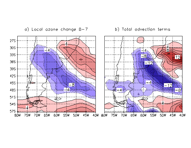
Figure 5: (a) Local ozone change from July 8^th to 7^th and (b) total (zonal, meridional and vertical) advection contributions to ozone changes integrated over the 100-30 hPa layer. Contour interval 2*10^-4 DU s^-1, all zero contours have been omitted.

The most simple transport ozone equation where the ozone-mixing ratio is conserved following the motion is:

where  stands for ozone mixing ratio, u and v are the horizontal wind components and  is the vertical velocity. Then multiplying by the appropriate quantities and performing a vertical integration of (1), ozone local changes between two close pressure levels may be obtained as the combined response of both horizontal and vertical transports of ozone mixing ratio integrated in the pressure layer.

In that sense, local ozone change between July 8^th and 7^th is shown in fig.5a while the contributions from zonal, meridional and vertical (total) advection terms integrated in the 100-30 hPa layer is shown in fig.5b. Both fields are in good agreement although the total advection field overestimates ozone local changes by approximately a factor of 1.7. This may be due to: a) the poor estimates of the vertical velocity field in the stratosphere, which may be very low compared to the real ones. b) The limitation of the mapping technique itself for levels above 30-hPa, although the analysis of SBUV/2 profiles over the region indicate that the contribution to local ozone changes came from the 125-62.5 hPa layer, with secondary contributions coming from both 62.5-37 hPa and 250-125 hPa layers. c) The transports taken only from 100 to 30-hPa, which may be misrepresenting the real situation.

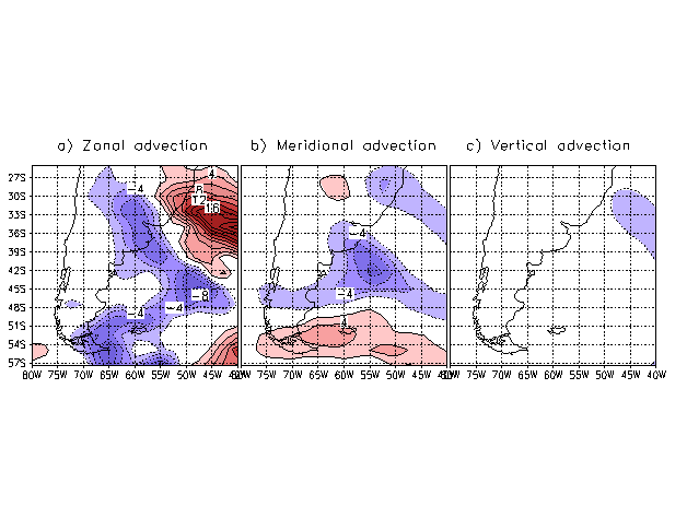
Figure 6: Contribution to total advection for July 8^th to 7^th from (a) zonal, (b) meridional and (c) vertical motion fields; each integrated over the 100-30 hPa layer. Contour interval 2*10^-4 DU s^-1, all zero contours have been omitted.

For the same day, each component of the total advection term integrated over the 100-30 hPa layer is shown in fig.6. Negative local ozone changes over the central part of Argentina and extending south-east to the Atlantic ocean are due to the combined contribution of both zonal and meridional advection. Meanwhile, the positive ozone changes located to the north of Uruguay and eastern Atlantic come from the zonal advection term partially offset by meridional and little vertical advection. To the eastern part of Tierra del Fuego and over 57ºS, 55ºW too much negative values are produced by the zonal advection term, although ozone changes over the region are positive (fig.5a).

4.c Lineal multivariate regression model

Suggesting that total ozone variability on synoptic time-scales is mostly explained by quasi-columnar motion of air along isentropic surfaces, Salby and Callahan (1993) derived a linear regression model that relates total ozone content to tropopause pressure and potential vorticity. In order to test this hypothesis and to find suitable predictors for ozone distribution, the following relationship was proposed:

where  is total ozone,  represents the tropopause pressure,  stands for the potential vorticity on isentropic surfaces of 315ºK, 330ºK and 450ºK, and , i=0, 4 are the corresponding regression coefficients.

To find the regression coefficients that fit the relationship given by (2), data from the entire month of 1994 July was used according to least square method. Then, (2) was resolved for the grid points of the SH when the corresponding time series of the variables involved have no gaps within the month. As an example, figure 7a shows the time evolution of the relative contributions from terms in (2) averaged over 35º-55ºS, 50º-70ºW, an area that encloses the eastern part of southern SA. Contributions from all terms (tropopause pressure and the sum of potential vorticity contributions) are in very good agreement with almost over the whole month, excepting in the period July 25^th to 30^th when the differences between each curve become the largest (about 28 DU). Apart from some few days at the beginning of the month, potential vorticity remains the main contributor to , while an analysis of potential vorticity terms discriminated for isentropic surfaces (fig.7b) shows that  pv₃₁₅  is the most important term, which in turn is comparable to tropopause pressure contribution.

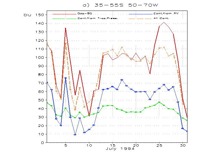
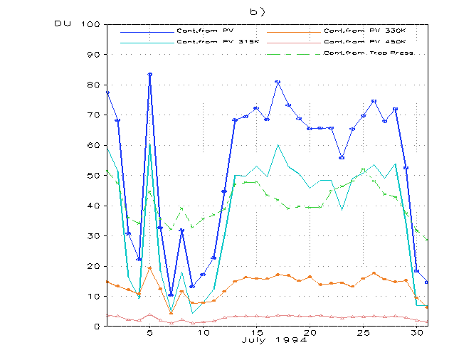
Figure 7: Time evolution of contributions from the different terms in (2). (a)    is represented by the continuous curve in red; contribution from tropopause pressure is labelled in green while that belonging to the sum of all potential vorticity at 315ºK, 330ºK and 450ºK is denoted by blue. The long dashed orange line represents the sum of all contributions (from tropopause pressure and potential vorticity). (b) Individual contributions from potential vorticity at 315ºK (light blue curve), 330ºK (orange) and 450ºK (rose); the sum of all this contributions are labelled in blue while contribution from tropopause pressure (green long-dashed) was plotted for comparison purposes.

For July 8^th, figure 8 presents: (a) field, and the contributions from: (b) the sum of potential vorticity from the three isentropic levels and (c) the tropopause pressure over southern SA. In particular, over the western Pacific, southern Patagonia and Malvinas Islands, and the band extending from the continent at 43ºS into the Atlantic Ocean to the east, relatively low values of the field are mainly due to decreased tropopause pressure (figs.8c-4f) and relatively low potential vorticity (figs.8b-4i). On the other hand, high values of over north of Uruguay and southeastward over the Atlantic (fig.8a) are due to relatively low potential vorticity (fig.8b-4I) and tropopause pressure enhancement (fig.8c-4f) both linked to a cyclone evolution over the area.

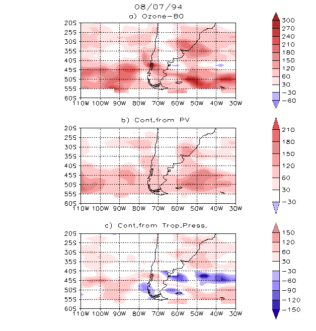
Figure 8: (a)  field, and the contributions from (b) the sum of terms of potential vorticity from 315ºK, 330ºK and 450ºK, and (c) tropopause pressure. Contour interval is 30 DU.  

5. Conclusions

In this paper, July 1994 extratropical total ozone field is comprehensively explored over time scales ranging from monthly to synoptic. The structure of stationary ozone field shows a clear signature of wave number 1 at middle-to-high latitudes with a minimum well above the climatological mean over southern SA. This minimum seems to be related to enhanced stationary atmospheric activity over the region, as well as to a subpolar jet maximum displaced westward over the southern Atlantic. For middle to low latitudes (up to 25ºS) ozone stationary fluctuations are determined by "tropopause effect".

Transient ozone fluctuations were also analysed in relation with upper-tropospheric wave activity. Mayor zones of standard deviation of ozone daily perturbations are shown to coincide with the regions of maximum standard deviation of 300-hPa geopotential height perturbations, although the former usually attain their maximum slightly poleward and downstream. In particular, southern SA display a maximum of both ozone and geopotential height standard deviation in association with the presence of a quasi-stationary, equivalent-barotropic ridge centered near 55ºS, 90ºW.

During July 7^th to 10^th a transient ozone wave evolving along subpolar jet latitudes was modulated and maintained by atmospheric activity. In order to determine the relative dynamical contributions from atmospheric waves to ozone distribution two approaches were pursued. Firstly, ozone local daily changes were explained in terms of a simple ozone transport equation and by use of the mapping technique. This approach yielded results that although overestimate local ozone changes, were able to reproduce comparable spatial patterns. The second approach proposed a multivariate linear regression model that relates ozone content to tropopause pressure and potential vorticity on isentropic surfaces. Results suggested that these quantities are valid predictors for ozone field; the most important contribution given by the potential vorticity on 315ºK and by tropopause pressure.

Acknowledgements

The authors are grateful to Dr.W.Randel for his helpful suggestions. Also we would like to thank specially to Dr.L.Flynn from NOAA/NESDIS for providing the SBUV/2 data. This work was partially supported by UBA Grant JX80 and by PICT 07-03781.

References

Andrews, D.G., J.R.Holton, and C.B.Leovy, 1987: Middle Atmosphere Dynamics. Academic Press, Inc. 489pp.

Berbery, H. and C., Vera, 1996: Characteristics of the Southern Hemisphere winter storm track with filtered and unfiltered data. J. Atmos. Sci., 53, 468-481

Salby, M.L., and P.F.Callaghan, 1993: Fluctuations of Total Ozone and Their Relationship to Stratospheric Air Motions. J.Geophys.Res., 98, 2715-2727.

Vigliarolo, P., Vera, C., and Díaz, S., 2000: Southern Hemisphere winter ozone fluctuations. In press at Quart.J.Royal Met.Soc.