Previous: Existence of the layered disturbances Next: Backward trajectory analysis Up: Ext. Abst.
3. EOF analysis
To examine appearance pattern of the layered disturbances, we
made an EOF analysis of time series of $v'$ amplitude averaged
in the dominant height region of 8-16km. The result suggests that
there are two dominant principal components. Figure 2 shows the
two dominant EOF components. The first component (EOF1) is characterized
as disturbances dominant at stations in the middle of Japan (30-37N,
referred to as EOF1 stations), and the second one (EOF2) is as
at stations in the south of Japan (23-30N, referred to as EOF2
stations). The time series of each EOF component has quite high
correlation (greater than 0.7) with $v'$ amplitude time series
at stations with high score, indicating that EOF1 and EOF2 modes
describe well the appearance of the disturbances at EOF1 and EOF2
stations, respectively.
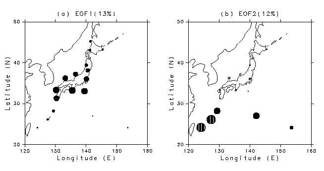
Figure 2. A pattern of (a) EOF1 and (2) EOF2 components. Positive and negative
values are indicated by closed and open circles, respectively.
The diameter of the circles is proportional to EOF values.
Using both radiosonde data and NCEP reanalysis data, the background
field preferred by the layered disturbances was examined. For
convenience, cases with values of EOF1 time series are greater
(less) than its standard deviation are referred to as positive
(negative) EOF1 cases. Similarly positive and negative EOF2 cases
are defined. Figure 3 shows composite of meridional cross sections
along a longitude of 135E for positive EOF1 and EOF2 cases. One
of the most interesting results is that EOF2 disturbances are
dominant when and where the background potential vorticity (PV)
is quite small. This suggests that EOF2 disturbances are due to
inertial instability.
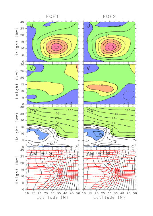
Figure 3. Composite of meridional cross sections along a longitude of 135E
of zonal (U) and meridional winds(V), potential vorticity (PV)
and (d) angular momentum (AM:black contours) and potential temperature
($\theta$: red contours) from top to bottom for positive EOF1
(left) and positive EOF2 cases (right). Contour intervals are
10{\ms} for U, 5{\ms} for V, and 0.1$\times$10$^{-9}$m$^2$s$^{-1}$
for AM. Units for $\theta$ are K. Contour intervals for PV are
0.025, 0.05, 0.1, 0.2, 0.4, 0.8, 1.6, 3, 6, 12, 25, 50, and 100PVU
(PVU$\equiv$10$^{-6}$Km$^2$kg$^{-1}$s$^{-1}$). The regions with
PV values smaller than 0.1PVU (greater than 1.6PVU) are colored
by blue (green).
To examine the frequency of inertial instability, the percentage
of time periods with negative PV values is calculated at each
grid point on the 345K surface where layered disturbances are
dominant for winter periods. The result is shown in Figure 4.
Surprisingly, the frequency of negative potential vorticity is
higher than 30 % in the zonally elongated region at 23-29N in
the western Pacific on 345K surface (an about 10km altitude).
This region corresponds to the locations of EOF2 stations. It
is interesting that such a high frequency of negative potential
vorticity is not observed at other longitudes in this latitude
region.
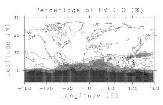
Figure 4. A contour map of the percentage of times when potential vorticity
is negative at each grid point in winter periods on an isentropic
surface of 345K. Contour intervals are 10%. The regions with percentages
greater than 20% are shaded. The region with larger percentage
is more darkly shaded.
Previous: Existence of the layered disturbances Next: Backward trajectory analysis Up: Ext. Abst.