• Introduction
• Existence of the layered disturbances
• EOF analysis
• Backward trajectory analysis
• Summary

FIGURES

• Figure 1
• Figure 2
• Figure 3
• Figure 4
• Figure 5
• Figure 6
• Figure 7

1. Introduction

Radiosonde observations of temperature and horizontal winds have been made at many stations in the world operationally over decades mostly for the purpose of weather prediction. Horizontal wind and temperature data obtained from operational high-resolution radiosonde observation in Japan have recently been available. By analyzing the data over 4 years at all 18 stations, it is discovered that clearly layered and long lasting structure in horizontal winds appears frequently in winter at several stations simultaneously. In this study, appearance patterns and sources of the layered disturbances are also examined by EOF analysis and backward trajectory analysis, respectively.

2. Existence of the layered disturbances

A typical example of the layered disturbances is shown in Figure 1. Figure 1a shows original (i.e. unfiltered) meridional wind $v$ at Naha located in the south part of Japan. Strong and shallow northward winds are observed below the upper tropopause continuously from 25 December to 10 January. To see the layered structure of meridional winds more clearly, we extracted fluctuations using a bandpass filter in the vertical with cutoff lengths of 1.5 and 6 km and a lowpass filter in time with a cutoff length of 2 days, which hereafter we refer to as $v'$ component. Similar disturbances are seen simultaneously at other stations of Ishigakijima (Figure 1c) and Chichijima (Figure 1d).

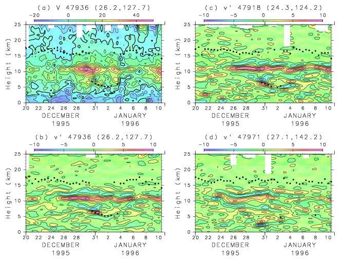
Figure 1. Time-height sections for the time period of December 20, 1995 to January 10, 1996 of (a) $v$ at Naha (26.2N, 127.7E, station No. 47936), (b) $v'$ at Naha, (c) $v'$ at Ishigakijima (24.3N, 124.2E, 47918), and (d) $v'$ at Chichijima (27.1N, 142.2E, 47971). Contour intervals are 5{\ms} ($\cdots$, -10, -5, 0, 5, 10, $\cdots$) for (a) and {\ms} ($\cdots$, -5, -3, -1, 1, 3, $\cdots$) for (b), (c), and (d). Thick contours show 0{\ms} for (a). Dots indicate the tropopause levels.

Such layered disturbances frequently appear at many stations mostly in winter. Thus, further examination is made for winter periods from 1 December through 10 March in each year. The total number of analyzed vertical profiles is 802 at each station. It should be noted that such small vertical-scale atmospheric disturbances have been analyzed mostly in terms of gravity waves so far. However, it may be needed to consider another possibility of inertial instability particularly for small-scale disturbances in low latitude regions.

3. EOF analysis

To examine appearance pattern of the layered disturbances, we made an EOF analysis of time series of $v'$ amplitude averaged in the dominant height region of 8-16km. The result suggests that there are two dominant principal components. Figure 2 shows the two dominant EOF components. The first component (EOF1) is characterized as disturbances dominant at stations in the middle of Japan (30-37N, referred to as EOF1 stations), and the second one (EOF2) is as at stations in the south of Japan (23-30N, referred to as EOF2 stations). The time series of each EOF component has quite high correlation (greater than 0.7) with $v'$ amplitude time series at stations with high score, indicating that EOF1 and EOF2 modes describe well the appearance of the disturbances at EOF1 and EOF2 stations, respectively.

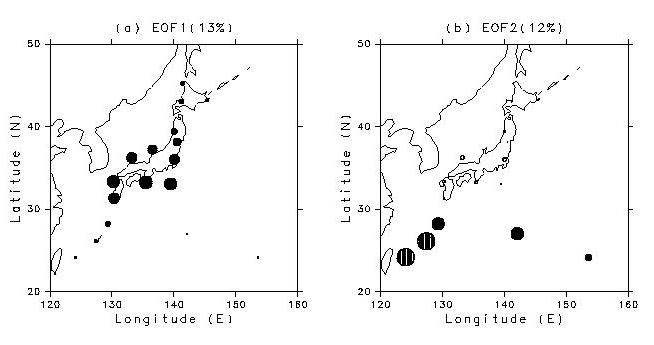
Figure 2. A pattern of (a) EOF1 and (2) EOF2 components. Positive and negative values are indicated by closed and open circles, respectively. The diameter of the circles is proportional to EOF values.

Using both radiosonde data and NCEP reanalysis data, the background field preferred by the layered disturbances was examined. For convenience, cases with values of EOF1 time series are greater (less) than its standard deviation are referred to as positive (negative) EOF1 cases. Similarly positive and negative EOF2 cases are defined. Figure 3 shows composite of meridional cross sections along a longitude of 135E for positive EOF1 and EOF2 cases. One of the most interesting results is that EOF2 disturbances are dominant when and where the background potential vorticity (PV) is quite small. This suggests that EOF2 disturbances are due to inertial instability.

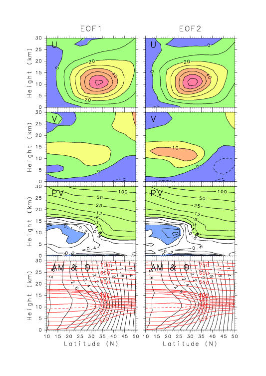
Figure 3. Composite of meridional cross sections along a longitude of 135E of zonal (U) and meridional winds(V), potential vorticity (PV) and (d) angular momentum (AM:black contours) and potential temperature ($\theta$: red contours) from top to bottom for positive EOF1 (left) and positive EOF2 cases (right). Contour intervals are 10{\ms} for U, 5{\ms} for V, and 0.1$\times$10$^{-9}$m$^2$s$^{-1}$ for AM. Units for $\theta$ are K. Contour intervals for PV are 0.025, 0.05, 0.1, 0.2, 0.4, 0.8, 1.6, 3, 6, 12, 25, 50, and 100PVU (PVU$\equiv$10$^{-6}$Km$^2$kg$^{-1}$s$^{-1}$). The regions with PV values smaller than 0.1PVU (greater than 1.6PVU) are colored by blue (green).

To examine the frequency of inertial instability, the percentage of time periods with negative PV values is calculated at each grid point on the 345K surface where layered disturbances are dominant for winter periods. The result is shown in Figure 4. Surprisingly, the frequency of negative potential vorticity is higher than 30 % in the zonally elongated region at 23-29N in the western Pacific on 345K surface (an about 10km altitude). This region corresponds to the locations of EOF2 stations. It is interesting that such a high frequency of negative potential vorticity is not observed at other longitudes in this latitude region.

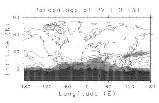
Figure 4. A contour map of the percentage of times when potential vorticity is negative at each grid point in winter periods on an isentropic surface of 345K. Contour intervals are 10%. The regions with percentages greater than 20% are shaded. The region with larger percentage is more darkly shaded.

4. Backward trajectory analysis

To see the origin of this anomalous potential vorticity, we made a backward trajectory analysis. Six hourly NCEP reanalysis data are used to make integration backward in time for 7 days with a fourth-order Runge-Kutta scheme. The time step is taken to be 1 h. The backward trajectories are calculated for each station as a starting location every 6 hours for the whole winter periods. The total number of trajectories is amount to 1464 for each station. Figure 5 is a typical example of positive EOF2 case. The negative potential vorticity air for EOF2 disturbances can be traced back to the equatorial region south of Japan within 3 days. This is due to a strong northward blanch of Hadley circulation associated with strong convection on the Maritime continent.

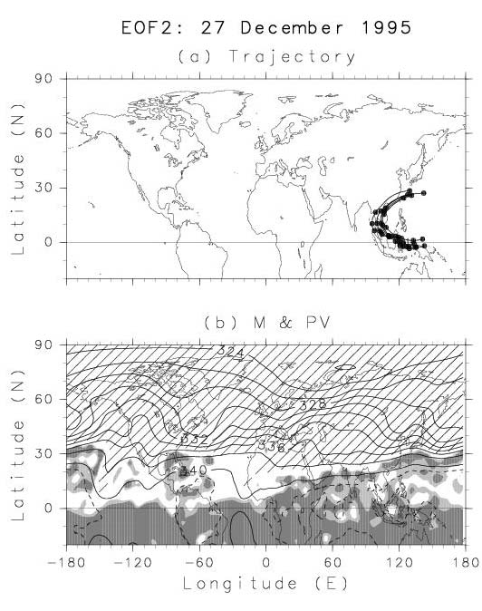
Figure 5. (a) Backward trajectories starting at EOF2 stations at 00Z 27 December, 1995. The distance between dots in each trajectory corresponds to 1 day. (b) A contour map of Montgomery stream function at 00Z 27 December, 1995. Contour intervals are 10$^3$ m$^2$s$^{-2}$. Dashed curves are the contours of 340.5$\times$10$^3$m$^2$s$^{-2}$. Darkly (lightly) shaded are the region with negative potential vorticity (smaller than 0.1PVU). The stratospheric regions (i.e. PV$>$1.6PVU) are hatched.

On the other hand, the background potential vorticity is low but not negative for EOF1 disturbances (Figure 6). Air parcels reaching EOF1 stations are traced back to far west because of the existence of strong westerly jet. Thus, it is inferred that the EOF1 disturbances are due to inertial gravity waves trapped in a duct of the westerly jet core.

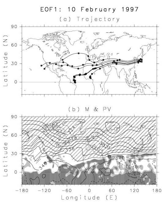
Figure 6. As in Figure 5 but for the time periods starting at 00Z 10 February, 1997.

Using all trajectories for the whole winter periods starting at each station, the number of trajectories getting to each grid point is calculated for each time lag (Figure 7). Contours show the same number (10) of trajectories for each radiosonde station. Line types of the contours are changed according to the EOF groups: black thick contours are for EOF2 stations, gray thick contours are for EOF1 stations, and thin contours are for remaining stations in the north part of Japan. It is seen that the trajectories are clearly divided into the EOF groups. Air parcels at EOF1 stations are traced back to farther west, which is likely due to the existence of strong westerly jet. Air parcels at EOF2 stations have different trajectories. Those are distributed southwest of Japan on Day -1, the distribution is elongated zonally on Day -3, and the distribution is spread more zonally in the equatorial region on Day -5. This fact supports the results of EOF analysis that EOF1 and EOF2 disturbances occur independently.

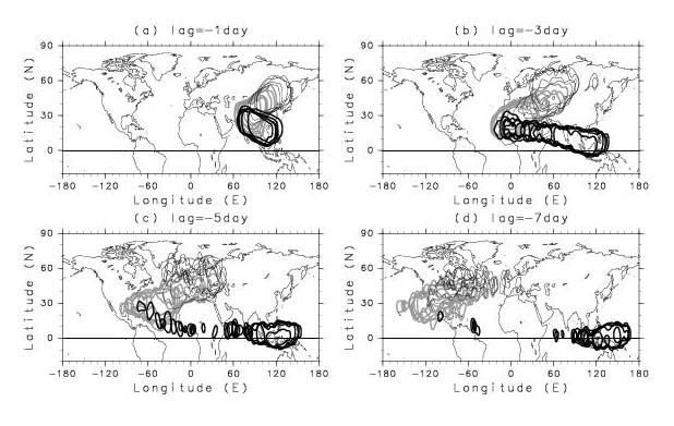
Figure 7. Contours indicating the region where the number of backward trajectories is 10, for day (a) -1, (b) -3, (c) -5., and (d) -7 starting at every radiosonde station in Japan.

5. Summary

By analyzing operational high-resolution radiosonde data in Japan over 4 years, it is revealed that long-lasting layered wind disturbances appear frequently in winter at several stations simultaneously. The dominant height region is 8-16km. The result of an EOF analysis indicates that there are two dominant modes for their appearance. The first component (EOF1) is dominant in the middle of Japan (30-37N), and the second (EOF2) dominant in the south of Japan (23-30N). The background fields for the layered disturbances are examined using NCEP reanalysis data. The background potential vorticity is frequently negative when and where EOF2 disturbances are dominant, suggesting that the EOF2 disturbances are due to inertial instability. The negative potential vorticity air for EOF2 disturbances can be traced back to the equatorial region within a few days. On the other hand, the background potential vorticity around EOF1 disturbances is low but scarcely negative. Air parcels at EOF1 stations are traced back to far west because of the existence of strong eastward jet stream. Thus, it is inferred that the EOF1 disturbances are due to inertia-gravity waves trapped in a duct of the westerly jet core.

This paper was submitted to J. Atmos. Sci.

K. Sato and T. J. Dunkerton, 2000: Layered structure associated with low potential vorticity in the upper troposphere and lower stratosphere revealed by high-resolution radiosonde observation data in Japan.