Previous: EOF analysis Next: Summary Up: Ext. Abst.

4. Backward trajectory analysis

To see the origin of this anomalous potential vorticity, we made a backward trajectory analysis. Six hourly NCEP reanalysis data are used to make integration backward in time for 7 days with a fourth-order Runge-Kutta scheme. The time step is taken to be 1 h. The backward trajectories are calculated for each station as a starting location every 6 hours for the whole winter periods. The total number of trajectories is amount to 1464 for each station. Figure 5 is a typical example of positive EOF2 case. The negative potential vorticity air for EOF2 disturbances can be traced back to the equatorial region south of Japan within 3 days. This is due to a strong northward blanch of Hadley circulation associated with strong convection on the Maritime continent.

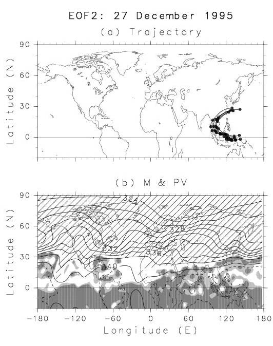
Figure 5. (a) Backward trajectories starting at EOF2 stations at 00Z 27 December, 1995. The distance between dots in each trajectory corresponds to 1 day. (b) A contour map of Montgomery stream function at 00Z 27 December, 1995. Contour intervals are 10$^3$ m$^2$s$^{-2}$. Dashed curves are the contours of 340.5$\times$10$^3$m$^2$s$^{-2}$. Darkly (lightly) shaded are the region with negative potential vorticity (smaller than 0.1PVU). The stratospheric regions (i.e. PV$>$1.6PVU) are hatched.

On the other hand, the background potential vorticity is low but not negative for EOF1 disturbances (Figure 6). Air parcels reaching EOF1 stations are traced back to far west because of the existence of strong westerly jet. Thus, it is inferred that the EOF1 disturbances are due to inertial gravity waves trapped in a duct of the westerly jet core.

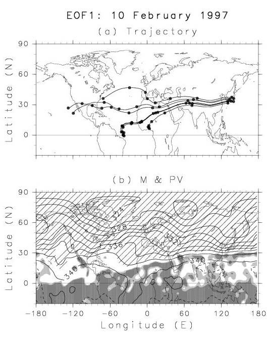
Figure 6. As in Figure 5 but for the time periods starting at 00Z 10 February, 1997.

Using all trajectories for the whole winter periods starting at each station, the number of trajectories getting to each grid point is calculated for each time lag (Figure 7). Contours show the same number (10) of trajectories for each radiosonde station. Line types of the contours are changed according to the EOF groups: black thick contours are for EOF2 stations, gray thick contours are for EOF1 stations, and thin contours are for remaining stations in the north part of Japan. It is seen that the trajectories are clearly divided into the EOF groups. Air parcels at EOF1 stations are traced back to farther west, which is likely due to the existence of strong westerly jet. Air parcels at EOF2 stations have different trajectories. Those are distributed southwest of Japan on Day -1, the distribution is elongated zonally on Day -3, and the distribution is spread more zonally in the equatorial region on Day -5. This fact supports the results of EOF analysis that EOF1 and EOF2 disturbances occur independently.

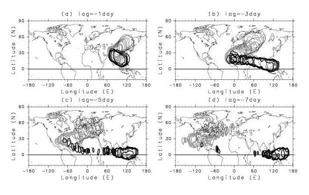
Figure 7. Contours indicating the region where the number of backward trajectories is 10, for day (a) -1, (b) -3, (c) -5., and (d) -7 starting at every radiosonde station in Japan.