A printer-friendly version of this document is available as a PDF file (80 kbytes).

Electric field for point-like charges

These notes are a wrapped-up version of the problem solved in the tutorial.

The problem: Assume you have three charges on the x-axis; from left to right they are $-3q, \, +q, \, +2q$. The distances between consecutive charges is $d$ (see the diagram for details).

Task: find the point(s) on the x-axis at which the electric field vanishes.

Let us try to figure out, on a diagram, in which regions on x-axis one may hope to find a point of $\vec{E}=0$. In what follows $E$ and $E_X$ will be used partially interchangeable; I hope this will not create confusion. Anyway, in our case on the x-axis one has $\vec{E} = E_X \hat{x}$, so the magnitude $E$ of $\vec{E}$ is the absolute value of $E_X$.

On the top of the diagram, in three rows, the $\vec{E}$'s generated by each of the charges is depicted. As you can see, the field created by $-3q$ is pointing toward the charge in all of the regions. The field created by the positive charges is ``outbound'' from the corresponding charge. To add some information, the magnitudes of the vectors are also indicated. The fields are calculated at the middle point of each interval, that is at $d/2$ of the adjacent charges. I also indicated the fields at the points which are at $d/2$ to the left of $-3q$ and to the right of $+2q$. The numbers on the arrows are the relative magnitudes of the fields - the unit magnitude is the value of $E$ generated by the $-3q$ at distance $d/2$ around it¹

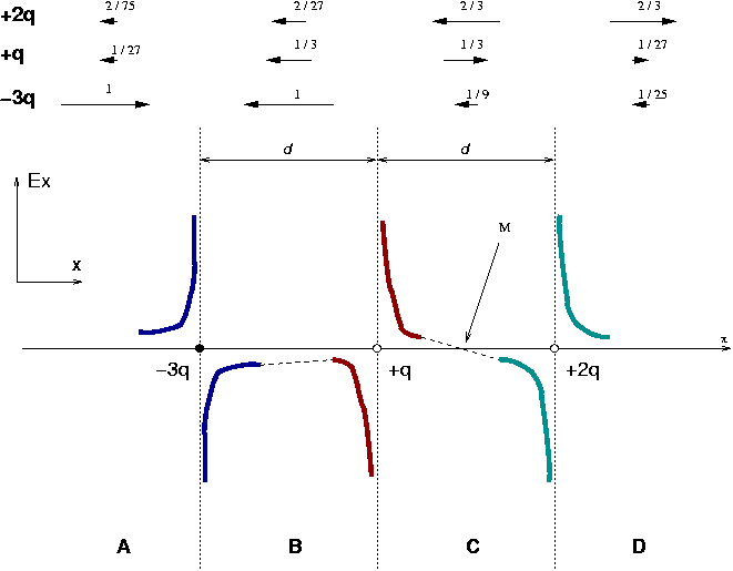
As one may notice, in region B the fields are all oriented in the same direction, to the left, therefore we should not expect the resultant field to vanish in that region. May we expect to find solutions in all other regions?

To check this, let us sketch the behaviour of the resultant $E_X$ in the vicinity of the charges. It is clear that close to a charge, the value of the field is mainly due to the charge sitting at that particular location. For example, at the point located at distance $\ell$ to the left of the $-3q$ charge, the projection on x-axis of the total field is given by²

$$E_X = + k_e\frac{3q}{\ell^2} - k_e\frac{q}{(\ell+d)^2} - k_e\frac{2q}{(\ell+2d)^2}.$$ (1)

Now, if one takes the limit $\ell \rightarrow 0$, the second and the third terms in (1) stay finite, while the first term blows up to infinity; therefore, the dominant contribution is from the charge in vicinity of which we calculated the field. With the same approach, you may convince yourself that the behaviour of $E_X$ is as depicted.

Since the value of the field is a continuous function of distance (except for the location of the charges, where ones gets singularities), we observe that in region C there must be a point M at which $E_X=0$.

What about regions A and D? The field apparently goes to 0 at large distances away from the charges. It can be shown that it is not vanishing at any finite distance in those regions. The proof is postponed to the end of this document. In conclusion, there is only one point of x-axis at which the field vanishes.

To find the position of M we choose the origin of the x-axis to be at the location of the $+q$ charge. Let the coordinate of M be $x$. Then the distances from M to the $-3q$ and $+2q$ charges are $d+x$ and $d-x$, respectively.

The field $\vec{E}$ on x-axis has only $E_X$ component. We require

$$E_X = k_e\left[- \frac{3q}{(d+x)^2} + \frac{q}{x^2} - \frac{2q}{(d-x)^2}\right] = 0,$$ (2)

where, again, the signs come from the orientation of the corresponding vector relative to the positive direction on x-axis - see also the footnote 1. Equation (2) gives

$$4y^4 -2 y^3 + 7y^2 -1 =0,$$ (3)

where for brevity I denoted $y\equiv x/d$. We expect the solution to obey $0 < y < 1$. Indeed, there is a unique solution with this property, namely $y=0.382902$. Hence we obtain $x \approx 0.383 d$. You may get this solution either numerically (using Mathematica, Maple, etc.) or by digging into math monography for the analytical solution of the 4-order polynomial equations.

Let us now prove that the field does not vanish in the A and D regions. In the textbook (Serway & Jewett) there is a similar problem, 19.15, dealing with the field generated by a dipole on its axis.

As before, we choose the origin of x-axis at the location of $+q$ charge, and find the expression for $E_X$ far away from the charges, say, in the region D. Let $x$ denote the position at which we calculate the field. For this situation we assume $d\ll x$, which is to say that

$$\xi \equiv \frac{d}{x} \ll 1.$$

We have

$$E_X = k_e\left[- \frac{3q}{(x+d)^2} + \frac{q}{x^2} + \frac{2q}{(x-d)^2}\right]$$

$$= \frac{k_e q}{x^2}\left[ - \frac{3}{(1+\xi)^2} + 1 + \frac{2}{(1-\xi)^2}\right]$$

$$\approx \frac{k_e q}{x^2}\left[ - 3(1-2\xi) + 1 + 2(1+2\xi)\right]$$

$$= \frac{k_e q}{x^2}\times 10\xi = k_e\frac{10qd}{x^3}.$$ (4)

Above we used the approximation , which is valid for $\alpha \ll 1$. In conclusion, we found that far from the region with charges, the field is proportional to $1/x^3$ - it goes to 0 as $x\rightarrow \infty$ but never vanishes for any finite $x$. As a sidenote, the $1/x^3$ dependence is typical for configurations of charges which have total charge equal to 0. See also 19.,15 in the textbook (Serway and Jewett).

Revised: 02/06/05 © 2005 Sorin Codoban