Disclaimer! ..."To err is human"... so please, don't take for granted my statements. Any hint/recommendation written here should be filtered through your common sense and compared with what you know from your own experience.
First advice: you have to follow the directions put forward in the announcements and guide sheets on the official site of the PHY110_138 Lab.
At the Lab test you are asked to take data, write a short report (of 1..3 pages - since you only have 15-20 min. for this task) and also draw by hand a graph (and a fit line) related to the experiment you're given.
Keep in mind that the TAs have little time (a few minutes) for grading each report, so make sure that your write-up is concise, clear, and more or less neat.
Unlike for the lab. write-up, there is no need to write extensive introduction, purpose, method and discussion sections. Write only what's essential for the reader to understand your results.I listed below those "items" I would like to find in a lab. test report.
Short introduction, purpose
Data taking, Table
Graph
Error in the slope and Error calculus
Conclusion
Short Introduction (Purpose)
Write a few lines about the goal of the experiment and the main steps to achieve it. For example, for the Boyle's Law you'd say something like:
"[...] we are going to test the validity of the Boyle's law for moderate pressure values (about 1..2 × atmospheric pressure).
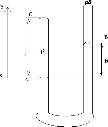
To prove that pV = const at constant temperature, we measure the length l of the air column (air trapped in the tube) and its pressure p by measuring the gauge pressure h (see the diagram).
Since V = l * S (where S is the cross section area of the tube ) and the pressure

(with the atmospheric pressure p0 = H mmHg) we see that checking pV=const is the same as showing that l(h+H)= const*
(the density of mercury and Sare assumed to be constant at constant temperature).To check this relationship we plot l(h+H) vs. l . We expect our data to fit to a horizontal line (i.e of slope 0)."
At this point you may want to draw a diagram (a sketch of the experimental setup), which shows also the quantities you're measuring.
A clearly labeled diagram helps a lot when TAs evaluate your work!
Make your notations clear!
The diagram should make your notations self explanatory!Data Table
The table should be announced in the write-up and labeled accordingly
(something like: "The (V vs. I) for the resistor", "Height and time readings", etc...)The header must be neat and large enough to contain at least:
-The name (and notation for) the variables
-The units
-The (reading) error.The body of the table should have enough columns to host:
-The number of the trial (take 4 ... 6 trials; check with the guide sheet provided)
-The values of variables as you measure them (don't use scratch paper!)
-The column for errors - in case the reading error is changing from one trial to another (so that you cannot quote it in the header).
This column (for errors) may be substituted by a clear statement before or after the table; something like: "the error in Y is z%" or "the error in Y is calculated with the formula ....."
NOTE - In most cases the reader (i.e. the TA) would like to see the error for each value clearly displayed. This column will also help you plot the values and their error bars.Moral: include a column for the errors in your data table!
The graph
Use PENCIL!
(you may use pen for writing down numbers, but not for drawing the axes, the fit lines and the data points)Use most of the page for the plot (say, no less than 70% of the surface).
Label the graph (title, your name, student ID) and don't forget the labels on the axes.
Put the units wherever they need to be!
Make sure you understand what kind of fit line you expect to get. In some cases your fit line should pass through the origin (the (0,0) point); in other cases the intercept of the fit line with the axes is somewhere else.
Display the error bars if they are " displayable " (i.e. the error is large enough to be seen on the scale of your plot).
Do NOT circle the points!
I'd suggest using tiny bullet or star signs to display the data on the graph paper, then draw the error bars with thin lines.The slope is the most common info you have to retrieve from the plot. Show how do you get it right on the graph. Label the triangle used in the process (with letters), write the definition of the slope, and the value you get for it, with proper units.
Error in the slope
Note: In some cases (say, Free Fall, etc.), when the fit line is not a horizontal one, the error bars may be too small to be represented on the graph.
On the other hand, if the fit line is expected to be horizontal then by zooming in the (vertical) scale it is always possible to have visible error bars (see Velocity of the sound in a gas (1-st plot option), Boyle's Law, etc)You have to show the extreme fit lines (when the slope is not supposed to be 0, those are the lines of minimum and maximum slopes) which gives you an estimate of the error in the slope. I'd suggest you draw them with dash (or/and) thin lines and use solid-thick line for the best fit line.
Attention: if the line of best fit is supposed to pass through (0,0) then the extreme fit lines should also pass through (0,0) !
Classical example: in the "DC Circuits" experiment, the line of best fit and the extreme fit lines must all pass through the (0,0) point in (V,I) co-ordinates.
Try to keep the graph neat!One more comment on the plotting techniques: if your points lay on the fit line very well and the error bars are too small to be displayed, then retrieving the error "by hand" from the slope of the fit line is not possible.
Also, you do not have time to play with the graph, nor to perform the "high accuracy trick" explained in the Lab. manual, pag. 136.However, there is always an error in the slope; a small one, but still, there is!
Why?
Because you always have a reading error when reading the length of the sides of the triangle used for the slope calculation!
For example, if you read the rise (say, 100mm) and the run (say, 150mm) from the plot with a reading error of 0.5mm ( = half of the smallest division on the graph paper) then your relative error in the slope is
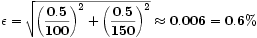
This tells us that no matter how well we perform the experiment (small reading errors, nice agreement of the data with the fit line, etc...) due to the method of retrieval of the slope from the hand-made graph, the relative error in the slope is at best, say, 0.3 - 0.5%.
Pretty surprising... :-)
Error calculus
This " item " has two sides:
(1) Reading errors
Almost every quantity encountered in the experiment has a reading error (and units!). Do not forget to quote them.
Example: t = ( 22.5 ± 0.3) oC
(2) Error propagation
Definitely, it is pretty hard to do any error propagation in those 15-20 min. But still, if you want an A (or higher) then you must attempt to do it.
Get an estimate of the error bars, plot them on your graph (see the end of the "Graph" section for what to do if the error bars are too small to be displayed).
Estimate by how much you may change the slope of your fit line (draw fit lines the min. and max. slope).
If the slope is expected to be 0 (like in Boyle's law exp., see above), then you can get an estimate of the error in that const* by shifting up and down the fit line, within the limits of the error bars.Read more about the fitting techniques in the Lab. Manual (pp. 133-141).
Example: in the Free Fall experiment, the fit line is
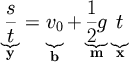
If your slope m turns out to be m=(4.85 ± 0.03)m/s2 then your g is
g=(9.70 ± 0.06)m/s2
N.B. Pay attention to correct error quotations
Good: (4.10 ± 0.03)*10-3 N/m; (1.70 ± 0.15) cm/s; (9.430 ± 0.004)mm
Bad: 4.1*10-3N/m ± 3.1*10-5 ; (1.7 ± 0.15) cm/s; (9.4300 ± 0.0041)mm
For more on error quotations, significant figures, propagation of errors and such, please read again the Error Assignment guide sheets