Disclaimer: ..." Any statement/recommendation on this page should be filtered through your common sense and compared with what you know from your own experience. Dont' take anything for the "ultimate truth"

Pay attention to the following steps:

• To show that pV = const. at constant temperature it is enough to show that
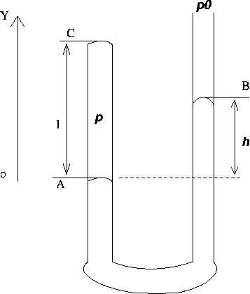
  l(h+H) = const^* at constant temperature. Here const^* is just another constant.

  Proof:
  p = d*g*h + p₀, where d is the density of mercury at room temperature, g is the acceleration due to gravity, h is the gauge pressure, and p₀ is the atmospheric pressure. Since p₀ can (and actually it is) expressed in mmHg as p₀ = d*g*H  , at the end we get that p = d*g*(h+H)
  On the other hand, V = (cross section area)*l. 
  Therefore, given that d and the cross section of the tube are constants during the experiment (this is true, provided the temperature is constant), the relationship p*V=const. is true if l*(H+h) = const^*.

  You may explain this (time permitting) in short, in the mini-introduction to your lab. test report.

• Draw a neat (large enough) diagram of the setup, with l, H and h properly labeled! For a better-looking diagram of the setup see the Boyle's law description (on UPSCALE).
• Show how do you calculate and measure:
  l   (the length of the air column) and
  h   (the gauge pressure).

  Note: pay attention to the sign of h . In some cases h   might be negative, but this should not scare you; the formula for the total pressure still involves the same (H+h) (it is always "+"  between H and h !). It just means that the pressure p is less than p₀, since now H+h < H .

• Pay attention to the design of the table, quotation of the (reading) errors right in the header, and make sure the units are quoted as needed.
• Be careful with the units.
  Note: h  and H  should have the same units when added!
  H is given in mm in the guide-sheet provided at the test..

• When plotting l*(H+h) vs. l choose the scale of the vertical axis such that the error bars for l*(H+h) are displayable.
  

  This can be easily achieved by performing a "blow up" of the region of interest.
  Say, if your values for l*(H+h) hover in the interval (2740, 2767)cm² then it's probably a good idea to take the vertical axis from 2700 to 2800 (cm²).
  The trick is to have enough room to display the points and the error bars. The relative errors are about 1% or less, as you may remember from the Boyle's experiment done during the year. Actually, you'd better check now which were your values for the relative errors.
  One needs to be able to plot values like (2740 ± 28)cm² and (2767 ± 28)cm²; that's why I've chosen the (2700, 2800) interval.

• Plotting [  l   vs. 1/(H+h) ] as a proof that pV is constant is NOT advisable, in my opinion.

  Note: you'll be given credit for this plot as well - but still, I'd suggest you avoid it. See my reasons below.

One may think that this kind of plot might be a "perfectly" viable alternative. Indeed, if one expects to have pV = const. then this means that V = const./p, or in other words l = const^* /(H+h). So, you expect to see this plot as a tilted line which, extrapolated, crosses the origin (0,0). In fact this plot is usually done during the regular lab. session of Boyle's law experiment, as a first step (to test the presence of a systematic error in l).

In my opinion this plot is NOT at all such a "perfect" alternative, especially when you draw the plot by hand (read: at the Lab Test).
I believe so, because on the plot l vs. 1/(H+h) you cannot display any error bars (because of the representation scale).
This also means you'll a have hard time in getting an estimate of how precise the Boyle's law holds (a task which is straightforward in l*(H+h) vs l  plotting; it's true that it requires a bit of extra work, but still...)
Therefore, avoid using the plot l vs 1/(H+h) for the "Boyle's law" at the Lab. test.

 

• You are NOT requested to give a numerical estimation of the pV (in Joules), as in the regular lab. experiment.
  I saw people doing that at previous Lab. tests. Why did they do that?! It doesn't prove anything more than l*(H+h)=const*, but gives the TAs a chance to complain about details (error propagation, etc...).
  I'm pretty sure you don't know the value of d at room temperature (or at 0^oC for that matter). So don't worry about computing pV in Joules!

• There are a few catches:
  The atmospheric pressure is given in mmHg at 0^oC (i.e. in torr), but you work at room temperature. You are not supposed to know the coefficient of volume expansion of the mercury, which is needed to correct the atmospheric pressure (in mmHg at 0^oC) to atmosp. pressure at room temperature.
  On the other hand the value of p₀ provided to you is a generic one (it might differ quite a bit from the atmospheric pressure you have during the experiment).
  Clearly, both these two factors affect the end-result. By how much.... well, that's another story.
  If interested, you may try in preparation for the test, to simulate using the fit program and your (real) Boyle's law data the effect of a wrong (lower or higher than the true value you had during the real experiment) atmospheric pressure on the end result.
  I know it sounds (too) complicated, but at least you'll have an idea whether or not you may blame this systematic error for the deviation of your result from the expected one :-)
• One expects to see the value of  const^*, i.e. l*(H+h) as your answer, quoted as
  ( Mean value ± Error ), in whatever units you may have.

  Your (best) guess for the mean value of l*(H+h) is close to the average of those 4 to 6 individual values that you get during the experiment.

  Note: you may check that usually, the line of best fit is not the one given by the average (see above remark)!
  It differs slightly. You may see this effect by playing around with the fit/graph program and your data. In any case, you should train your skills of guessing the line of best fit.

  However, the best fit line will cross the vertical axis at the position given by the average if you neglect the individual errors in the data points (imagine you set the error bars to 0). The error in the fit const^* will then be given by the standard error in the mean (recall the Error Analysis assignment....).

  The line of best fit does not cross the vertical axis at the average value because the data points with smaller errors are given more weight by the algorithm used by the fit program.

  
  Besides, one expects so see your conclusion (see below) on how well the Boyle's Law is verified.

  Note: It may happen that your points do not fit to a horizontal best fit line.
  This may occur either because you have some systematical errors (e.g. you measured incorrectly the height of the air column l) or because the Boyle's Law doesn't verify at the values of pressure and temperature you have.
  Although this worse case scenario may occur, in general you should expect that within error bars all your points lay nicely around a horizontal line of best fit. Check your notebook (plot done with the fit program), to see how your plot is supposed to look like.

• How precisely the Boyle's law is verified in your experiment is shown by the relative error, ε = Error / Mean, of your estimate for l*(H+h).

• For a fast track error calculation take your first and last pairs of (l, H+h ) values and calculate the error in the corresponding l*(H+h) values.

Most probably the errors for the intermediate points can be interpolated by an "educated guess". Be sure you explain that you calculated only the extremes and that you interpolated the errors shown for the inner points. If you have time, of course, you may calculate the errors for each set :-) (you only have 4 or 5 sets)

• The error  (E) in the end result (i.e. in the estimate of the mean of l*(H+h)) can be evaluated in a few ways:

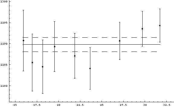
1) The recommended way of determining E  is by shifting up and down your horizontal fit line on the graph l*(H+h) vs l , and see by how much this can be done. The limits of this shift are given by the error bars you've plotted on the graph.
If the line of best fit is chosen correctly, then the shift is symmetric (see the sample plot) and the error in the mean is
E = (max value - min value) /2.
Here max value stands for the position of the top dash line on the above mentioned plot, while min value stands for the bottom dash line.

This seems to be the best method for the lab test !

A plot l*(H+h) vs. l   done with Faraday-based fit program will give you a good hint of how much you can shift the line of fit. Look after the dash lines the fit program draws above and below the best fit line. This kind of shift is what you have to do "by hand" at the Lab Test. Train yourself in advance!

2) Do the full error calculation ... not recommended, because of the time limitation!

 

• REMEMBER:  
  The most important thing for this experiment @ Lab. test is to show that l*(H+h) values can be fitted to a horizontal line with a good precision ( = small relative error ε), on a plot l*(H+h) vs l    (or l*(H+h) vs. 1/l, of l*(H+h) vs. (whatever changes), for that matter).
  This proves, as argued above, that pV=const. (at constant temperature) which is the Boyle's Law.
  The error calculus, although appreciated, is not the main point.

Last revised: July 02, 2003.
© Sorin Codoban, 2003.

Back to main page