| Short Introduction | Reading and Calibration Errors | Error bars ? | Conclusion
You are asked to use the "frictionless theory" of the free fall. Hence, the formula describing the motion of the body is:
s = v0 * t+ (g/2)* t 2
where s is the distance the body travels during the time t of the fall between the photogates, v0 is the initial velocity (at the 1st photo-gate), and g is the acceleration due to gravity.
Since retrieving "by hand" g from the parabolic shape described by the above s(t) relationship is neither an easy nor a pleasant task, we decide to perform a trick with the above formula, namely to divide both sides by t. We get a new expression
s/t = v0 + (g/2) *t
Now, the situation is much better, since a plot ( s/t vs. t) can be done and we expect to see it as a straight line. The line intersects the vertical axis at v0, and the slope is m = g/2 .
The reading and calibration errors
The reading error of the position of each gate is typically about 0.2 - 0.4 mm, (it's up to you what value to take). The distance s is the difference of coordinates of the two gates. Hence, the propagation of errors (be sure you write the right formula in your lab. test report) gives a reading error in s of err-s = (0.3 - 0.5) mm.
You are also advised that the calibration error of the meter tape is one part in 4000. This introduces an error of (s/4000) for each value of s.
Although the nature of the reading errors and calibration errors is different, you still may combine them in "quadratures" for this experiment because you don't know a priori if the calibration error acts with + or - (a systematic calibration error would act with one sign only; at least that's what common sense suggests).
The situation is nasty! It seems that my argument here is not quite correct, in the sense that nobody knows whether or not the calibration error in this experiment acts with +/- (as I tried to persuade you...) or just with "+" or just with "-".
For some reasons, " better known to itself", this experiment works out well if you combine the calibration and reading errors in quadratures...
Looks like the calibration error in our case acts as a "random" one, and shall be combined accordingly!
Details: I believe that most probably the calibration error enters with " + " for some values of s , " - " for others. It is the irregular stretching/squeezing of the measuring tape during manufacturing which gives this calibration error, and you don't know a priori which part is stretched or squeezed. Attention, this is only my guess, because otherwise it's hard to understand why in the Lab. Manual, Prep. Question no. 2 they ask you to combine the reading and calibration errors in quadrature (see below some more details).
Taking the above into consideration we get that
(Error in s) = Sqrt [(err-s)2 + (s/4000)2 ]
Someone (say, other TAs... at the lab. test...) may argue that combining the reading and the calibration errors is illegal. Of course this is a true statement in principle, but life is more complicated, as we've just seen.
Nevertheless, you are supposed to know that random errors cannot be combined with systematical ones in quadrature, so if at the interview you get into this be sure you are on "the right side of the force" :-).
Going back to the difference of two types of errors, in this experiment it's suggested that for small values of s you take err-s as your error while for large values (say, 1.5m an higher) you should take the calibration error alone as your full error.
In my opinion this is not the best option - it looks a bit artificial (and leaves errors for the intermediate s in the air: for example, how are you supposed to balance/combine the random reading error with the systematical one for s of about 1m ?)
At least for this particular experiment, given the probable nature of the accuracy (calibration) error, it's seems reasonable to combine all the errors in quadrature.
Regarding this side of the question see also the Lab Manual, Prep. Q. no. 2. for the Free Fall, in which it is suggested how the random and calibration error are to be combined. Be sure you understand how to deal with this error calculation.By the way, the numerical value of the error doesn't change that much, whatever recipe for the total error of the two discussed above you apply :-)
Moreover, as it will be shown below on this page, the error bars are too small to be represented on the hand-made graph. Nevertheless, it is important that you know that there is a difference in how one deals with different types of errors.Are the (reading) errors "displayable"?
Let us take a real-life example:
The range of values for s and t as taken from one (real) data set is s = (300 - 2300) mm and t = (100.0 - 500.0) ms.
Hence, the range of values for s/t would be (3 - 4.6) mm/ms.The error in s
For the smallest value of s the error is 0.4mm (I assumed a reading error of 0.3mm for the position of each gate and included the s/4000 error as well). Hence, the relative error is 0.4/300 = 0.0013 = 0.13%.
For the largest s value the error comes up to be 0.7mm. The relative error in this case is 0.7/2300 = 0.0003 = 0.03%.
An educated guess tells us that the relative error in s monotonically decreases as we move toward larger values in s.
N.B. Eventually (if we go with s up to 5m or so) the relative error will end up being only 1/4000 = 0.025%, due mainly to calibration error.
The error in t
Well, here we have a few options:
Shall we consider the error as only 0.05ms (the timer is a digital instrument, so the reading error's value is 1/2 of the last displayable digit)?
Or maybe a better option would be a reading error of 1-last-displayable-digit, so therefore in our case the error is 0.1ms.
Please, recall that during the lab hours I advised you to drop the plastic ball a couple of times for the same s to see if there is any fluctuations in the recorded time. Some of you did that, and indeed, in a few cases there was such an effect, so the "reading" error was taken to be 0.1ms.
It's up to you which reading error to take: 0.05 or 0.1ms. It might be even larger. Say, if you drop the ball a couple of times and see large fluctuations, then why not take it bigger? The experiment is the ultimate judge!
Just take care and EXPLAIN the reasons for your choice of error!
For the smallest time values the relative error would be 0.1 /100 = 0.001 = 0.1%.
For the largest time value the relative error is 0.1/500 = 0.0002 = 0.02%.
Again, an educated guess tells us that the relative error in time decreases as the value of t increases.
The error calculus for s/t
The relative error in s/t (ε) is given by
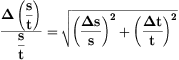
and has the values:For the smallest values of (s,t):
ε = 0.0016 = 0.16%.
For the largest values of (s,t):
ε = 0.00036 = 0.04%.
Summary:
The relative error in the s/t values ranges between 0.16% to 0.04%. These are rather small errors!
The absolute error in the s/t values is, accordingly, between 0.005 mm/ms to 0.002 mm/ms (first value corresponds to smallest value of s/t).What about the error bars?
Can we display any error bars for this experiment?
It might be that because of the scale used for the plot, no error bars can be shown!The range of values for s/t and t is
( 3.0 - 4.6 )mm/ms for s/t.
(100.0 - 500.0)ms for t.
Recall that we need to see the intersection with the vertical axis and that we expect to get a value of about (1.2 - 2)m/s = (1.2 - 2 )mm/ms for the v0 .
N.B. This is why I ask you to revise your lab. test experiments at least once, at home: so that you know ahead what you should expect to obtain!
We therefore estimate that the proper range for the vertical axis s/t is (1.0 - 5.0) mm/ms and for the horizontal axis t the range is (0 - 600.0)ms.
The size of the graph paper is about 18 x 25 cm. Let us take the long side for the (s/t) (say, we take 20cm for (5-1) = 4 mm/ms ) and the short side for the t (say, 18 cm for 600 ms.).
Therefore, on the vertical axis one millimeter of the graph paper corresponds to
A = 4 (mm/ms)/ 200 (divisions) = 0.02 mm/ms /division.On the other hand, on the horizontal axis you can display
B = 600 ms /180 (divisions) = 3.33 ms/division.Please, observe that I took into account that 1cm = 10 mm and that I assumed that 1 mm is the finest division one can see on the graph paper (well, you can probably see 1/3 of 1mm, but that doesn't change the outcome...see below).
Let us compare A and B with the error bars 'to be plotted' (if any!).
A = 0.02 mm/ms, but the error in s/t is at most 0.005 mm/ms (see above the estimates for the errors). No way to display it!
B = 3.33 ms but the error in t is only around 0.1ms. "Out of luck" again!
The moral:
The errors in s/t and t are both too small to be displayed! No error bars therefore!
Use Faraday's fit program (e.g. from home, via a web-browser) to graph or fit s/t vs. t.
See which are the typical results to be expected for v0, g and for the error in g.
About the errors: don't panic if your error in g (the error has to be retrieved from the graph) shows up a bit larger, by a factor of 2 or so, than what Faraday gives you.
Practice with Faraday's fit program using your (real) data.
See how the reading errors in s and t are related with the error in g.In your lab. test report try to answer the question:
Is the "accepted" value of g (9.80 m/s2) in the error interval (1-sigma) of the "experimental" value of g ?If you find that your g doesn't agree with the "real" g within the errors, it means that neglecting the friction (and using the frictionless theory to fit the data) wasn't such a good idea.
In fact, this is one of the questions for this Lab. test :-)Last revised: April 7, 2003
© Sorin Codoban, 2003