 |
Stratospheric Processes And their Role in Climate
|
||||||||
| Home | Initiatives | Organisation | Publications | Meetings | Acronyms and Abbreviations | Useful Links |
![]()
 |
Stratospheric Processes And their Role in Climate
|
||||||||
| Home | Initiatives | Organisation | Publications | Meetings | Acronyms and Abbreviations | Useful Links |
![]()
Description of statistical models
A varying amount of detail was made available regarding the statistical models used by the researchers in section 3.3 on the test data sets, and in section 3.5 on trend results. This section encapsulates the model information available. In some cases the particular model fitted impacts the trend results, as discussed in sections 3.3 and 3.5.
The models used for the primary text discussion on trends (section 3.5) are described more completely below. Following that, all model information is summarised in bullet form.
Logan and Megretskaia (Harvard model, sondes)
The model includes monthly means, four seasonal trends, a lagged QBO and a solar dependence. The monthly means are weighted by the inverse of the interannual monthly variance. The variances are computed with two iterations after fitting the model, to remove the variation due to the trend. The model does not account for autoregression. An intervention term is included in the model for the four Canadian stations at all pressure levels, at the date of the change from BM to ECC sondes; a similar term is included at Payerne for the tropospheric levels in April 1977 to account for the change in the time of soundings from ~1600 to 0930 (Logan, 1985). The QBO time series used is the 30 hPa winds for Singapore and the 10.7 cm solar radio flux at Ottawa/Penticton. Lags were determined for the QBO as described in Logan (1994). Percentage trends are calculated relative to the seasonal mean for the time series being analysed.
Tiao, Choi and Zhang (Chicago model, sondes)
The model includes monthly means, four seasonal trends, a lagged QBO, a solar dependence, and an intervention term as above for the Canadian stations and for Payerne. The residual noise is modelled as a first order autoregressive model, with different variances in different seasons. The QBO time series is the average of 50 hPa winds at Singapore, Balboa, and Ascension Island. The model assumes zero trend before Jan. 1, 1970. Outliers are removed; these are points whose residuals are more than three standard deviations away from the model fit. Percentage trends are calculated relative to the seasonal intercept in 1970 (or beginning of series if later) adjusted for solar effects, and intervention if used.
Hollandsworth and Flynn (SBUV and TOMS total)
The basic regression model for SBUV trend analysis in this report is of the form:
O3(t) = m (t) + A(t)X(t) + B(t)Xqbo(t-l) + C(t)Xsolar(t) + N(t)
This model is fitted to weekly ozone data in section 3.5, but
monthly data for the trend comparisons on the test data sets in
section 3.3. Here m (t) is the seasonal cycle, represented by a constant and 4 harmonics
(9 terms); ![]() is the seasonally-varying trend coefficient.
The trend proxy
is the seasonally-varying trend coefficient.
The trend proxy
![]() is time (time=0 at 1/1/78) and the coefficient varies
with 2 seasonal
harmonics (5 terms);
is time (time=0 at 1/1/78) and the coefficient varies
with 2 seasonal
harmonics (5 terms); ![]() is the seasonally-varying QBO
coefficient. The QBO proxy is the
30-hPa monthly-mean zonal-mean Singapore wind, lagged in time
with respect to the ozone values by up to a quarter cycle (backward
or forward) to produce the minimum residuals. The QBO lags are
a function of latitude and altitude. The coefficient varies with
one seasonal harmonic (3 terms); C(t) is the seasonally-varying
11-year solar cycle coefficient. The solar cycle proxy is the
5-week smoothed 10.7 cm solar radio flux. The coefficient varies
with one seasonal harmonic (3 terms). The full model has 20 terms.
There is no seasonal weighting, and autoregressive noise is taken
into account in the standard errors via a jack-knife refitting
method.
is the seasonally-varying QBO
coefficient. The QBO proxy is the
30-hPa monthly-mean zonal-mean Singapore wind, lagged in time
with respect to the ozone values by up to a quarter cycle (backward
or forward) to produce the minimum residuals. The QBO lags are
a function of latitude and altitude. The coefficient varies with
one seasonal harmonic (3 terms); C(t) is the seasonally-varying
11-year solar cycle coefficient. The solar cycle proxy is the
5-week smoothed 10.7 cm solar radio flux. The coefficient varies
with one seasonal harmonic (3 terms). The full model has 20 terms.
There is no seasonal weighting, and autoregressive noise is taken
into account in the standard errors via a jack-knife refitting
method.
Newchurch and Yang (Umkehr)
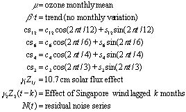
The trend model used to estimate the annual ozone trends from the Umkehr data is a uniform (non-seasonal) trend model of the form:
O3(t) = m + cs12 + cs6 +cs4 + cs3 + b .t + g 1Z1(t) + g 2Z2(t-k) + N(t)
where:

The model is an AR(1) autoregressive one, fit using multiple regression, and with the AR(1) parameter varying by month.
For the test data sets, however, Newchurch and Yang fit a monthly trend model for the TOMS and Uccle data for comparison to other researchers’ results. For reasons discussed in the text, they reported results from a seasonal trend model (based on fitting seasonal ozone averages) for the SAGE test data. In both cases, the solar and QBO effects were omitted for the test data sets.
Wang and Cunnold (SAGE trends)
The SAGE trend estimates result from the statistical model of Wang et al. (1996) with two significant differences. First, the model used here includes a seasonal modulation term where the Wang et al. model assumed none. Second, this model uses an exogenous series (Singapore winds) for the QBO coefficient, where the Wang et al. model used a fixed 28-month period. The linear regression model for the ozone trend is then:
O3(t) = A.t + Seasonal + C .QBO + D.Solar + N(t)
where:

Note: the QBO phase lag is determined by the maximum correlation between the 30 hPa Singapore zonal wind and the residual N(t) (fitted without QBO term)
Model summary
For easy comparison, here are the main features of the trend models in bullet form (ordered alphabetically by first researcher):
Bishop:
Fioletov:
Hollandsworth and Flynn:
Logan and Megretskaia (Harvard model):
McCormack and Hood:
Newchurch and Yang:
Randel:
Reinsel (only TOMS test data was submitted):
Tiao, Choi and Zhang (Chicago model):
Wang and Cunnold:
Ziemke and Chandra:
![]()