 |
Stratospheric Processes And their Role in Climate
|
||||||||
| Home | Initiatives | Organisation | Publications | Meetings | Acronyms and Abbreviations | Useful Links |
![]()
|
Stratospheric Processes And their Role in Climate
|
||||||||
| Home | Initiatives | Organisation | Publications | Meetings | Acronyms and Abbreviations | Useful Links |
![]()
2.4.1.1. Density Comparisons
Information on sites used for this study is given in Table 2.3. As before, SAGE II ozone densities less than 5x10¹¹ or greater than 1x1013 cm-3 were not used in doing the comparisons and the time filtering criteria presented in Table 2.2 were adopted. The SAGE II/sonde differences for 10 stations are shown in Figure 2.9 a to j. In general, the differences are small (3 to 5%) near 25 km but they increase with decreasing altitude reaching values from -5 to nearly -30% depending upon the site.
|
|
|
|
|
|
| Boulder |
|
|
|
|
| Hohenpeissenberg |
|
|
|
|
| Uccle |
|
|
|
|
| Hilo |
|
|
|
|
| Payerne |
|
|
|
|
| Lauder |
|
|
|
|
| Tateno |
|
|
|
|
| Sapporo |
|
|
|
|
| Edmonton |
|
|
|
|
| Goose Bay |
|
|
|
|
Table 2.3: Ozonesonde Stations to compare with SAGE. CI is Carbon-Iodine; ECC is Electrochemical Concentration Cell; BM is Brewer-Mast.
2.4.1.2. Latitude Variations of the Differences
Figure 2.10 shows the SAGE II/sonde differences for selected altitudes at each station plotted as a function of the integral of the SAGE II aerosol extinction. The integrated aerosol extinction is calculated by integrating the SAGE II altitude dependent extinction data (version 5.96) collected at the times of the coincidences in altitude and averaging over the time period of the coincidences. The linear fits to the data in Figure 2.10 show strong negative slopes at all altitudes which are significant at the one sigma level. The reasons for this correlation are unknown, but could be either aerosol algorithm correction effects or altitude registration errors.
Possible Algorithm Errors:
Accurate retrieval of ozone densities at altitudes below about 19.5 km (the exact altitude depends on the aerosol loading and its variation with altitude) is dependent on the accuracy achieved in removing aerosol extinction from the 0.6 m m channel used by SAGE II for ozone sensing. The aerosol extinction at 0.6 m m is extrapolated using Mie theory from measured aerosol extinctions in the other SAGE II channels. Ozone errors will depend in a non-linear way on errors in aerosol extinction.
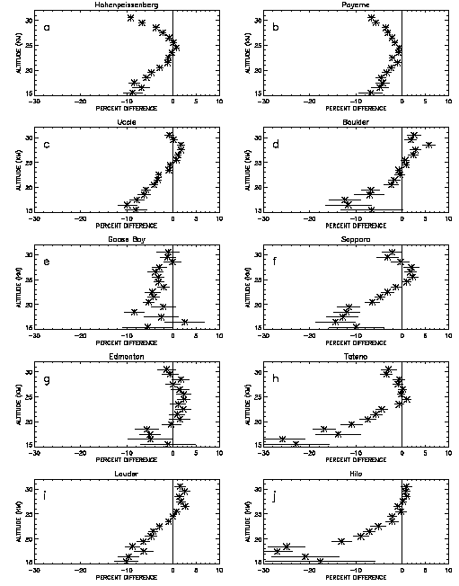
Figure 2.9. Percent differences between sonde and SAGE II ozone at 10 sites. Information on the site locations is given in Table 2.3.
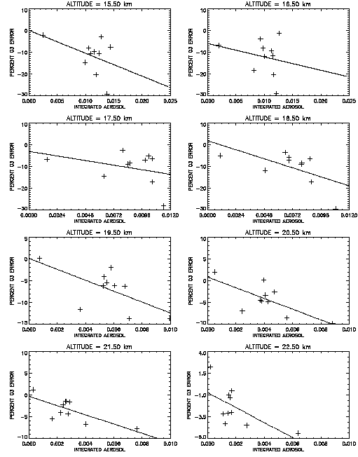
Figure 2.10. The percent differences between sondes and SAGE II as a function of the integrated aerosol extinction at various altitudes.
Possible Altitude Registration Errors:
An alternative explanation for the latitudinal difference (see Chapter 1) postulates the existence of altitude registration biases in the SAGE II data in the 15 to 20 km region. The biases, which may be as large as 0.5 km, are most likely caused by errors in the SAGE II solar edge detection algorithm in the presence of a strong gradient in the 1.02 m m extinction profile, which is the channel most sensitive to aerosol extinction. An altitude registration error would give an incorrect removal of Rayleigh scattering extinction from the 0.6 m m channel and therefore produce errors in the ozone determination.
2.4.1.3 Trends of Sonde Minus SAGE II Differences
Trends of sonde minus SAGE II differences as a function of time are calculated by a simple linear regression. Figure 2.11 shows an example difference time series for 20.5 km at Hohenpeissenberg along with the fitted line. The positive slope means that the sonde ozone values are increasing with time relative to the SAGE II data. The difference vector has an auto-correlation coefficient of less than 0.2 and thus the individual data points are independent. The slope of the fitted line in Figure 2.11 is 0.68 ± 0.38%year-1 where the uncertainty is the 2 sigma error on the slope.
The altitude dependent trends in the SAGE II/sonde differences are shown in Figure 2.12 for the eight stations used later in Chapter 3 to compare SAGE II and sonde trends. These stations cover the latitude range from 36oN to 56oN. The trends of differences at individual stations vary widely in comparison to SAGE II. In the 20 to 25 km region the trends of differences vary from -1.7%year-1 at Edmonton to +1%year-1 at Sapporo. At lower altitudes, the variations are larger, ranging from values greater than -2%year-1 At Sapporo to about 3%year-1 at Boulder (although not significant at the 2 sigma level).
Another way to compare the data is to combine the matched pair differences from all eight stations into one data set, construct a time series at each altitude, and calculate the trend of the differences. These results are shown in Figure 2.13. Analysing the data in this way gives small but non-significant trends of differences (£ 0.3% ± ~0.3 to 0.5%year-1) at all altitudes except 15.5 km where the value is about 0.83± 0.6%year-1, 2s . It was decided to combine the matched pair differences from the various stations in this way because of the small number of coincidences at the lower latitude stations in the set. An alternate method would be to average the ozone change differences from the eight stations. This would give larger overall differences and would weight the stations with fewer coincidences the same as those with a large number of coincidences. Because the data used in Figure 2.13 are matched points differences at each station, spatial effects are not important.
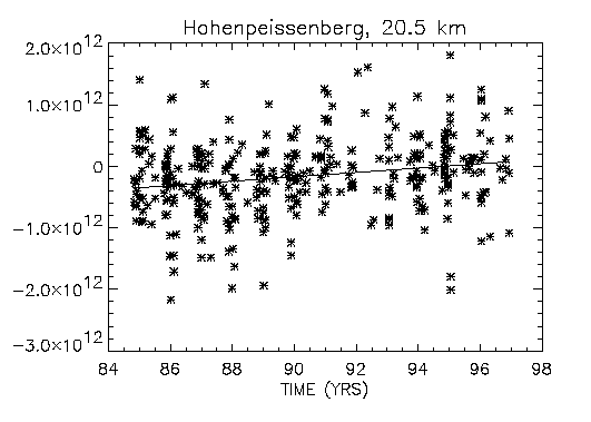
Figure 2.11 Differences in sonde minus SAGE II ozone as a function of time for Hohenpeissenberg at 20.5 km.
2.4.1.4. Summary and Conclusions
SAGE II/sonde ozone comparisons (see Figure 2.9) reveal small differences in the 25 km range, but differences increase with decreasing altitude, reaching maximum values of nearly 30% at two of the ten sonde sites. The sites with the largest differences are generally those where the low altitude ozone densities are smallest. There are at least two explanations for the altitude dependence of the differences between sonde and SAGE ozone measurements shown in Figure 2.10: algorithm issues or altitude registration errors. The sonde/SAGE II comparisons themselves do not shed light on the causal mechanism for the differences.
Trends of sonde minus SAGE II differences at individual sonde sites show large variability and care should be taken in using SAGE II ozone data to calculate ozone trends in narrow latitude ranges. On the other hand, using the combined data set covering the latitude range from 36 to 56° N and above 15.5 km, the trend of the differences are £ 0.3%/year (none of which are significant to the 2 sigma level except at 19.5 km). At 15.5 km, the largest difference occurs at 15.5 km where it is about 0.8%year-1 and is statistically significant.
Extensive intercomparisons between stratospheric ozone lidars and the SAGE II instrument are presented in this section. Table 2.4 summarises the location of the lidar sites, the lengths of the lidar time series, and the institutions of the eight lidar teams participating in this study.
2.4.2.1. Difference Time Series
Time series of differences between lidar and SAGE II measurements were calculated for each site at 10 altitude levels : 15, 17.5, 20, 22.5, 25, 30, 35, 40, 45 and 50 km. The differences are formulated as (Lidar-SAGE)/SAGE and are given in %. No vertical scale or units conversion was necessary since the SAGE II and the ozone lidars provide ozone vertical profiles in the same units. The SAGE II data correspond to algorithm version 5.96. The matching criteria for selecting the SAGE II measurements around each site was ±2.5° in latitude, ±12° in longitude and ±24 hours or ±48 hours coincidence. The GSFC measurements were performed at various locations since this instrument is a mobile system designed for intercomparisons with other ozone or temperature lidars involved in the NDSC (Network for the Detection of Stratospheric Change); so the differences for the GSFC lidar correspond to various sites; GSFC, TMF, OHP, Hawaï and Lauder. Depending on the experimental systems, the whole altitude domain is not covered by all the lidar systems. Also, the altitude range covered can change over the length of the lidar data record due to improvements which allowed the measurements to be extended in altitude (e.g. implementation of Raman channels as discussed in Chapter 1). The altitude range can vary from one lidar site to another, depending on the meteorological conditions or the power of the laser sources. Both the SAGE II and the lidar measurements were perturbed in the lower stratosphere by the volcanic aerosol cloud emanating from the Pinatubo eruption. SAGE II data were screened to accept only data with errors lower than 12% in the low stratosphere. Most of the lidar systems, which did not include Raman channels could provide valid measurements only above the volcanic cloud. The upper altitude of the cloud reached 30 km or more in the fall of 1991 and decreased steadily with a time scale of about 8 months afterwards. Due to decreases in signal-to-noise ratio of the lidar signals with altitude, the resolution of the lidar measurements is lower in the upper stratosphere (generally above 40 km) requiring that the resolution of the SAGE data be degraded to match the lidar resolution in this altitude range.
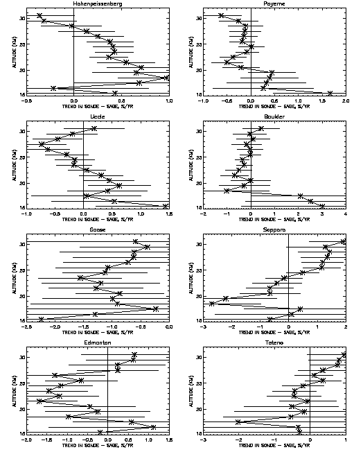
Figure 2.12. Trends in the sonde-SAGE II ozone differences as a function of altitude for eight sonde stations between 35° N and 53° N. The bars are 2 Standard Error.
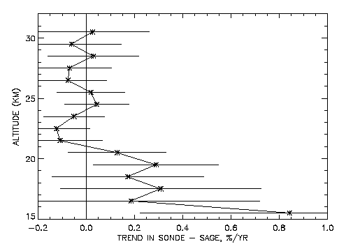
Figure 2.13 The altitude dependence of the trend in the sonde - SAGE II differences for the combined coincidences of the eight sonde sites shown in Figure 2.12.
|
|
|
|
|
| RIVM | Lauder |
|
|
| DWD | Hohenpeissenberg |
|
|
| SA-CNRS | OHP |
|
|
| NIES | Tsukuba |
|
|
| MRI | Tsukuba |
|
|
| NASA GSFC | mobile instrument |
|
|
| JPL | TMF |
|
|
| JPL | MLO |
|
|
Table 2.4: Lidar stations
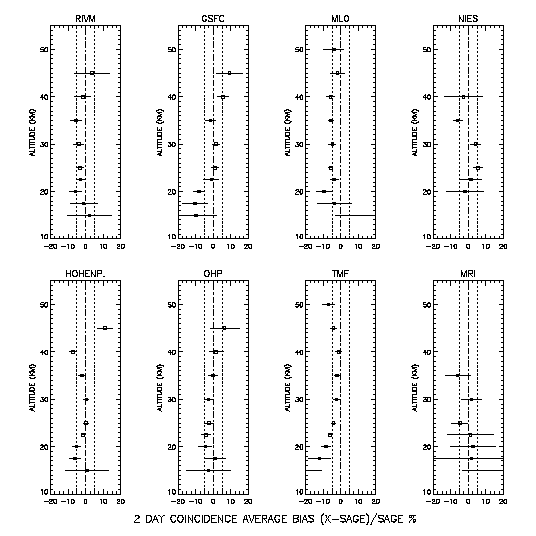
Figure 2.14. Average difference between the lidars and SAGE II as a function of the altitude for the ±2 day coincidence criterion. The error bars correspond to two sigma standard error.
2.4.2.2 Absolute Differences as a Function of Altitude
As in Section 2.4.1, first the results of the absolute differences are presented to an indication of the confidence level that can be placed on trend values. The vertical profile of the average differences for the two day coincidence criterion is displayed in Figure 2.14, together with the two sigma standard error and the number of coincidences. The results for one day coincidences occasionally show some small differences in the average values and the corresponding error bars but these differences do not change the global picture of the results for the various data sets. The number of coincidences (see Table 2.5) is highly variable from one station to the other, depending on the length of the time series and the frequency of the measurements. The maximum number of coincidences for each station ranges from 10 (MRI) to 190 (DWD) for the two day coincidence criterion. Four stations provide more than a maximum of 50 events: DWD, OHP, TMF and GSFC.
The best agreement between ozone lidars and SAGE II is found between 22.5 km and 35 km. In this altitude range, the average difference is slightly negative and sometime significant at the two sigma standard error confidence level, but it generally does not exceed ±5%; the largest differences are observed in the MLO time series (tropics), where the negative bias stays around -5% from 25 km to 40 km. In the lower stratosphere, the variability is much larger at 15 km and some biases exceeding 20% in absolute value are found (MRI, TMF and MLO) but the lidars and SAGE II generally agree within the two sigma level. Around 20 km, the average difference is generally negative and significant with values ranging from -4.5 ±3.7% to -9.5 ± 4.1%, except for the Japanese stations where it is smaller. These results, like the sonde comparisons discussed in Section 2.4.1, raise a note of caution about using SAGE data for trends in the lower stratosphere below about 20 km. Above 40 km, the average difference increases and can be positive (DWD, GSFC) or negative (TMF, MLO). The 50 km altitude is hardly reached by the lidar measurements, except by the TMF and MLO instruments.
|
|
|
|
|
|
|
|
|
|
|
|
|
|
|
|
|
|
|
|
|
|
|
|
|
|
|
|
|
|
|
|
|
|
|
|
|
|
|
|
|
|
|
|
|
|
|
|
|
|
|
|
|
|
|
|
|
|
|
|
|
|
|
|
|
|
|
|
|
|
|
|
|
|
|
|
|
|
|
|
|
|
|
|
|
|
|
|
|
|
|
|
|
|
|
|
|
|
||
|
|
|
|
|
|
Table 2.5: Number of lidar - SAGE II coincidences for the various stations
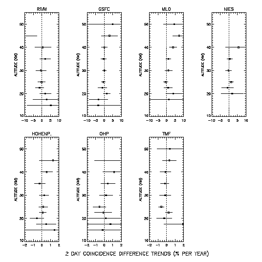
Figure 2.15. Trend of the average difference time series (± 2 days coincidence). The error bars correspond to the two standard error value of the trend.
2.4.2.3. Trends of Lidar - SAGE Differences
Trends of the difference time series are displayed in Figure 2.15 as a function of altitude, for each station and for the two day coincidence criterion. The error bars correspond to the two sigma standard error of the trend. Again, the results are not significantly different from the one day coincidence, so only the two day coincidence results will be discussed here. Likewise, the analysis focuses on the stations and altitude levels characterised by a number of coincidences large enough to provide reliable results on trends. Note that the scale on Figure 2.15 has been increased to ±2% in the case of Hohenpeissenberg, OHP and TMF.
In most cases, the lidar-SAGE difference time series show generally no trend significant at the two standard error confidence level. Due to the higher variability of ozone at altitudes below 20 km, the standard deviations are higher in this altitude range, and in general, the trends of the differences are larger than 1%year-1. The only exceptions are for the OHP and Hohenpeissenberg time series, which show non-significant trends of < 1%year-1. The trends are also higher above 40 km, due to decreases in the lidar measurement signal-to-noise. In these regions the trends generally exceed 1%year-1. Over the 22.5 km to 35 km interval, the trend does not exceed 0.5 ±1%year-1 on average. Values less than 0.3%year-1 with standard errors not exceeding 0.4% are found in the case of the longest records.
2.4.2.4. Comparative Study of Lidars and SAGE II Changes Over the Entire Time Period
As another approach, difference of trends comparisons were done at each station determined by calculating the trend for each time series separately (SAGE II and lidar) without trying to match observations in time. The length of the data record used was defined by the shortest time series (the lidar in all the cases). The changes considered here correspond to a simple linear fit to the data points without removing the seasonal variations. The SAGE II data were selected according to the same spatial criteria as in the previous paragraphs (±2.5° in latitude and ±12° in longitude). Since the seasonal variation was not removed from the data, care was taken to calculate the changes over exactly the same period of time. However, due to the sampling of the SAGE II measurements at each site, some differences can arise, especially in the case of short time series. For some of the longer time series (DWD and OHP), significant differences in the trends are found around 20 km. In the case of the DWD lidar, significant differences are seen at 20 and 22.5 km, where the change is negative for the lidar while for SAGE II, it is positive at 20 km and slightly negative at 22.5 km. At 20 km, the difference reaches -1.6 ±1%year-1. Concerning the OHP time series, a significant difference of -1.4 ±1.1%year-1 is observed at 20 km, where both instruments show a negative trend (larger in absolute value in the case of the lidar). Since the previous section showed that the SAGE II trends could be verified to about 0.5%year-1 by these two lidars, such differences should be checked with a more elaborate trend model.
2.4.2.5. Summary and Conclusions
The comparison between 8 lidars and SAGE II shows general agreement in absolute ozone density values for both types of measurements especially in the middle stratosphere (25-35 km). Poorer agreement is obtained in the lower stratosphere probably due to atmospheric variability and in the upper stratosphere (above 35 or 40 km, depending on the instruments) due to the lower signal-to-noise of the lidar measurement. Using coincidence time series corresponding to the 48 hours criterion and based on more than 40 events, the non significant average differences range from (-1.6 to 1.7)± 3% (two sigma standard error) in the middle stratosphere. The significant biases found in this altitude range are always negative (with the SAGE values being high with respect to the lidar data) and range from (-2.4 to -5.6) ±1.5%. Differences are largest on average in the southern hemisphere mid-latitude and northern hemisphere tropical stations. In the lower stratosphere, SAGE shows a positive bias with respect to the lidar especially at 20 km where it ranges from (-4.5 to -9.5) ±4%. At 15 km, no significant bias is generally observed but large differences exist and the variability is much larger.
Concerning possible drifts of SAGE II with respect to the lidars determined using matched coincidence events, the trends in lidar minus SAGE II differences for the longer coincidence times series (DWD, OHP, TMF) show generally non significant slopes in the 22.5 - 35 km altitude range varying from (0.1 to 0.5) ±0.4%year-1. The shorter coincidence time series generally indicate trends within 1.5 ±1.5%year-1. Below 20 km, the trends of the longer coincidence times series are within 1% to 2%year-1 and the two sigma uncertainty increases to 1% per year on average.
In summary, based on the SAGE II - lidar comparisons, the SAGE II trends from 20 to 35 km can be validated to about the 0.5%year-1 level. Below 20 km, although there is, in general, no statistically significant drift between SAGE II and the lidars the standard errors of both the absolute differences and the trends of differences are larger. Atmospheric variability is high in this range and the number of long-term records is smaller. According to the longest record, the SAGE II trends could be validated only to about 1%year-1 down to 17 km.
2.4.3.1. Introduction
The Umkehr data used for the analysis in this chapter came from the World Ozone and Ultraviolet Radiation Data Center (WOUDC) where they were all inverted in March 1997 from N-values using the Umkehr inversion algorithm [Mateer and DeLuisi, 1992] employing the uniform Sx error covariance matrix. This study further restricted the population of retrievals to those with small differences between observed and fitted N values (rmsres £ 1.3 N units) and with convergence criteria feps £ 0.15 and dfrms £ 0.01 in the inversion process. For such Umkehrs, the difference between observed and retrieved total column ozone is less than 1 DU in two-thirds or more of the retrievals. All Umkehr values are reported on the Bass and Paur [1985] scale. Table 2.6 lists the 19 Umkehr stations, grouped in broad latitude intervals, considered in this analysis, along with the record length of station observations within the 1979-1996 satellite period. The table also lists the fractional number of months represented within that period and the fraction of the Umkehrs available from the WOUDC database that passed the stringent convergence-criteria tests. Calculations performed in the Chapter 3 trends analyses indicate that the more restrictive convergence criteria do not significantly affect the computed trends from these Umkehr stations. Nevertheless, to insure the highest quality coincidence-comparison results, we applied the more stringent criteria to the Umkehr/SAGE comparisons reported in this chapter. The SAGE I data are altitude corrected according to Wang et al. [1996]. The SAGE II data are version 5.96. For all SAGE data, we omit ozone values with error estimates greater than 50% and also omit observations with an anomalous flag set to true; however, we do not screen any data based on aerosol amounts, which may affect the SAGE results below 20 km (layer 4).
Because aerosols in the lower-stratospheric aerosol layer affect the UV radiation scattered down from the zenith sky during the Umkehr observations, these aerosols cause retrievals of ozone in the upper stratosphere (primarily in layers above layer 6, that is > 30 km, i.e., well above the aerosol-layer altitude) to be underestimated during periods of high aerosol loading [DeLuisi, 1979]. Two different Umkehr aerosol corrections are applied separately through the analysis; the theoretically derived correction is described in Mateer and DeLuisi [1992], while the empirical correction is described in Newchurch and Cunnold [1994] and Newchurch et al. [1995, 1997]. At each station, for the population of measurements coincident with SAGE observations, we calculate the layer-mean ozone differences ±2 sem for individual Umkehr layers 4 through 8, layers 2+3+4 combined, layers 8+9+10 combined, and the columns for layers
|
|
|
|
North |
|
|
|
|
|
| Northern mid-latitude | ||||||||
|
|
|
|
|
|
|
|
|
|
|
|
|
|
|
|
|
|
|
|
|
|
|
|
|
|
|
|
|
|
|
|
|
|
|
|
|
|
|
|
|
|
|
|
|
|
|
|
|
|
|
|
|
|
|
|
|
|
|
|
|
|
|
|
|
|
|
|
|
|
|
|
|
|
|
|
|
|
|
|
|
|
|
|
|
|
|
|
|
|
|
|
|
|
|
|
|
|
|
|
| Tropics | ||||||||
|
|
|
|
|
|
|
|
|
|
|
|
|
|
|
|
|
|
|
|
|
|
|
|
|
|
|
|
|
|
|
|
|
|
|
|
|
|
|
|
| Southern mid-latitudes | ||||||||
|
|
|
|
|
|
|
|
|
|
|
|
|
|
|
|
|
|
|
|
|
|
|
|
|
|
|
|
|
|
|
|
|
|
|
|
|
|
|
|
| Antarctica | ||||||||
|
|
|
|
|
|
|
|
|
|
Table 2.6: Information concerning Umkehr stations considered in this study including station number, name, country, latitude, longitude, record length within the SAGE I/II (1979-1996) study period, fraction of month observed during the study period, fraction of observations that passed the more stringent inversion convergence criteria, and comment regarding whether the station was compared to SAGE I/II or reason that it was not compared.
4-10, 3-10, and 2.10. These layers and layer combinations derive from the Umkehr retrieval averaging kernels, which indicate the altitude and extent of the information content of this method [Mateer and DeLuisi, 1992]. We also calculate the linear regressions separately for the Umkehr, SAGE, and differences of coincident pairs of Umkehr-SAGE time series for all layers and combinations of layers expressed in both percent per year and Dobson Units [DU] per year ±1s confidence interval on the linear regression slope. The layer-mean ozone differences and the linear regression slopes are also separately plotted as a function of layer. All of these quantities are calculated separately for two time-difference criteria, 24 and 48 hours, and for the two aerosol corrections. We then average, within broad latitudinal ranges, the layer-mean ozone differences, layer regression slopes, and the regression slopes of the coincident differences for stations considered suitable for comparative analysis.
2.4.3.2. SAGE and Umkehr Time Series
As an example of the results at an individual station, Figure 2.16 shows the time series of Umkehr observations coincident with SAGE I and SAGE II in all specified layers and layer combinations plus the total ozone column indicated as layers 1+…+10. The regression lines are simple, linear fits to the data; they are not trend calculations in that they do not take into account any external influences (solar, dynamical, etc.) nor seasonality nor autocorrelation. These particular data were corrected for optical aerosol interference using the Mateer and DeLuisi factors. Using the Newchurch et al. aerosol corrections makes no significant (1s ) difference in the regression slopes in any layer or combination of layers; however, the two corrections differ by approximately 2% in the average column ozone amounts. The close correspondence of the two independent aerosol correction methods enhances our confidence in the applicability of both methods for trend calculations. However, because the Mateer and DeLuisi factors conserve total column ozone, we recommend using those factors. These small differences between the aerosol correction methods are characteristic of all stations. Figure 2.17 shows quantities analogous to Figure 2.16 Umkehr measurements, but for the SAGE I and II observations. There is no aerosol correction applied to the SAGE data in these analyses. Because SAGE rarely measures ozone in layer 1, the layer 1-10 total-column time series is not shown. The data missing in both the Umkehr and SAGE time series result from missing SAGE observations and, therefore, missing coincidences (although the Umkehr data are complete in all layers). The persistent data gap between late 1981 and late 1984 results from the missing SAGE observations between the end of SAGE I and the beginning of SAGE II. Figure 2.18 shows the differences (in DU) between the Umkehr and SAGE at individual coincidences plus the linear regression through those differences. The uncertainties for all slopes in Figures 2.16 through 2.18 are 1-s confidence intervals. Regression slopes calculated for the SAGE II period only (not shown) and projected through the SAGE I period fit the SAGE I period well, supporting the conclusion that the SAGE I and SAGE II instruments are well calibrated with respect to each other. Because Figure 2.18 results from differences of coincident pairs of observations, secular geophysical variations are intrinsically accounted for and resulting regression slopes significantly different from zero indicate real differences between the two measuring systems.
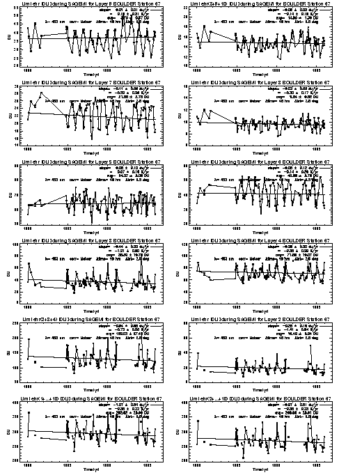
Figure 2.16 Time series of layer-ozone retrievals from Umkehr observations at the Boulder station coincident with SAGE I/II measurements. Panels display individual layers 2 through 9 and combinations layers 1 through 10, 2 through 10, 2+3+4, and 8+9+10 as indicated. The slope of the linear regression +/- 1 s.d. in DU year-1 and %year-1 (as a fraction of the indicated average layer-ozone amount) along with the maximum allowed time separation (48 hr) and latitude separation (2.5 degrees) are indicated. Umkehr ozone amounts were corrected for aerosol effects using the Mateer and DeLuisi [1992] factors.
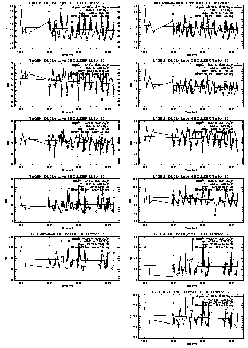
Figure 2.17 As in Figure 2.16, but for the SAGE I and II observations. Because SAGE rarely observes ozone in layer 1, the panel representing combined layers 1 through 10 is omitted. The data gap from 1982-1985 occurs between the end of SAGE I and the beginning of SAGE II.
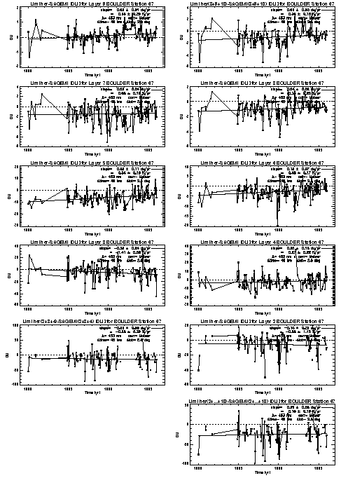
Figure 2.18 As in Figure 2.16, but for the differences (Umkehr - SAGE) in DU of the individual coincident pairs.
2.4.3.3. Layer-mean ozone and regression slopes
Figure 2.19 presents the layer-mean ozone differences ±2 standard errors of the mean (2 sem) during the SAGE I/II period for the 48-hour time intervals and the Mateer and DeLuisi aerosol correction method. The layer averages of 2 southern-hemisphere stations, Lauder and Perth, appear in panel (a), while the layer averages of 6 northern-hemisphere stations, New Delhi, Cairo, Tateno, Boulder, Haute Provence, and Belsk, appear in panel (b). Neither a more restrictive 24-hour time requirement nor an alternate aerosol correction method significantly affects these results. In the northern-hemisphere results, one can see significant SAGE-high biases in all layers, except layer 4, resulting in column biases of 7±1% for the Mateer and DeLuisi aerosol correction (5±1% for the Newchurch aerosol correction). The SAGE-high biases in layers 2 and 3 result from the ozonesonde climatology that forms the Umkehr a priori profiles. These a priori profiles dominate the Umkehr retrieval in the lower layers. This bias is also consistent with the direct SAGE-ozonesonde comparisons in this report. The column biases are essentially the same as the column biases between Umkehr and SAGE version 5.93 reported by Newchurch et al. [1997], although the vertical structure varies somewhat from station to station, especially in the upper layers. Therefore, the average vertical profile of layer-mean biases depends, somewhat, on which stations are included in the average. SAGE II version 5.93 is the publicly available version at the time of this report. Version 5.96 will be made available by the time of the publication of this report. Differences between allowed time separations between 24 and 48 hours are not significant. The combination layers 2+3+4 results are plotted at level 3.5 and the layer 8+9+10 results appear at level 8.5 both in larger, disconnected symbols. The southern-hemisphere results possess very similar structure and magnitude, but larger variances.
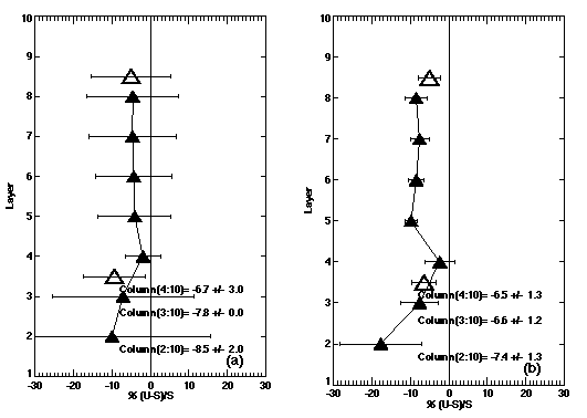
Figure 2.19. Layer-mean ozone differences expressed as Umkehr-SAGE I/II in percent ±2 sem of SAGE I/II layer-mean amounts for individual layers 2 through 8 (solid triangles), combined layers 2+3+4 (open triangles) plotted at layer 3.5, and combined layers 8+9+10 (open triangles) plotted at layer 8.5 for stations Perth (32° S) and Lauder (45° S) in the southern hemisphere in panel (a) and stations New Delhi (29° N), Cairo (30° N), Tateno (36° N), Boulder (40° N), Haute Provence (44° N), and Belsk (52° N) in the northern hemisphere in panel (b). Average differences ±2 standard errors of the mean for column amounts 2.10, 3-10, and 4-10 are also indicated. Coincident criteria are 2.5 ° latitude and 48 hours. All Umkehr observations are individually corrected for aerosol interference using the Mateer and DeLuisi correction factors.
Figure 2.20 displays the regression slopes of the Boulder station (as a typical example) for both 24-hour coincidences (squares) and 48-hour coincidences (circles) plotted against layer. Panel (a) presents the regression slopes of the Umkehr observations, panel (b) presents the slopes of the SAGE I/II observations, and panel (c) presents the slopes of the coincident-pair differences (Umkehr-SAGE). The large, disconnected symbols at level 2.5 represent the regression slopes of the layer 2.10 column amounts; the symbols at level 3.5 represent the layer 2+3+4 amount slopes; and the symbols at level 8.5 represent the layer 8+9+10 amount slopes. Smaller connected symbols represent individual layers. Results for both allowed time separations plotted together with 1-s uncertainties reinforce the similarity of these two time criteria. The Boulder Umkehr slopes are between 0.0 and 0.7%year-1, depending on layer and SAGE I/II slopes are nearly constant at 0.5%year-1 above layer 3. The slope uncertainties are consistent between Umkehr and SAGE measurements and also between time coincident criteria.
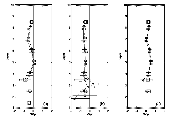
Figure 2.20 Regression slopes (%/year) of the layer-ozone time series of coincident observations ±1s confidence interval about the regression slope for the Boulder station (40° N, 255° E) . Panel (a) shows the slopes of the Umkehr observations; panel (b) shows the slopes of the SAGE I/II observations; and panel (c) shows the slopes of the coincident-pair differences (Umkehr-SAGE) within 2.5° latitude and 24 hours (squares) or 48 hours (circles). The disconnected open symbols represent layers 1 through 10 plotted at layer 1.5 (Umkehr only); layers 2 through 10 plotted at layer 2.5; layers 2+3+4 plotted at layer 3.5; and layers 8+9+10 plotted at layer 8.5. The connected symbols represent individual layers 2 through 8 for SAGE and 4 through 8 for Umkehr. All Umkehr observations are individually corrected for aerosol interference by using the Mateer and DeLuisi aerosol correction factors.
The results of these analyses indicated that certain stations should not be used for comparison to the SAGE regression slopes either because the coincidence density was too low or because discontinuities in the time series would produce anomalous discrepancies without intervention analysis. Indications for the 19 stations considered here are listed in Table 2.6. Because we chose not to remove the level shifts with interventions, these stations are not included in the latitudinal averages of layer-mean ozone nor averages of the regression slopes.
The northern mid-latitude (NML) average regression slopes and associated 95% confidence intervals appear in Figure 2.21 for Umkehr (panel a), SAGE I/II (panel b), and the coincident-pair differences Umkehr-SAGE (panel c). Panels (a) and (d) show the average slopes ±2 standard errors of the mean (i.e., an estimate of the variance between stations) of the Umkehr observations; panels (b) and (e) show the average slopes of the mean of the SAGE I/II observations; and panels (c) and (f) show the variance-weighted average slopes ±95% confidence intervals of the coincident-pair differences (Umkehr-SAGE within 2.5° latitude and 48 hours). The variance-weighted 95% confidence interval (also shown) is calculated as 2 [(S s i -2) -1]1/2, where s i is the standard deviation of the regression slope of an individual station time series. The largest discrepancy between Umkehr and SAGE regression slopes (panel c) occurs in layers 8 and 8+ where the slope of the coincident-pair differences is 0.3±0.2%/year, significantly different from zero at the 95% confidence level. In all other layers and layer combinations, the absolute slope of the differences is less than or equal to 0.2±0.2%/yr. Similarly, the slopes expressed in DUyear-1 present a consistent picture between Umkehr and SAGE observations, on average. The analogous figures for the southern mid-latitude (SML) averages appear in Figures 2.21 panels d, e, and f. The southern mid-latitude averages show marginally significant discrepancies between Umkehr and SAGE only in layers 7 and 8+. The vertical structure of the SAGE/Umkehr differences in the variance-weighted SML averages is similar to the NML results. Primarily due to the smaller sample size, the uncertainties in the SML are somewhat larger (~0.3%/year) than the uncertainties in the NML averages.
The 95% confidence-interval uncertainty in the total-column proxy (layers 2 through 10) regression slopes is on the order of 0.2%/year in the NML where the Umkehr/SAGE slope differences are not significantly different from zero and on the order of 0.3%/year in the SML where the slope differences are also zero. This close correspondence between SAGE and Umkehr total columns and ozone profiles suggests a fundamental agreement over time between these two measurements systems with some variation in the vertical distribution of the regression slopes at the 95% confidence level of 0.2%/yr.
2.4.3.4. Summary and Conclusions
In summary, we find significant layer ozone-amount biases (Umkehr lower than SAGE) increasing from 2±5% (2 standard errors of the mean) in layer 4 to 8±3% in layers 5 through 8 resulting in significant column (layers 2.10) biases of 7±1% (Umkehr lower than SAGE I/II). These layer-ozone biases differ by approximately 2% as a function of the 2 independent aerosol correction schemes employed. Comparisons of regression slopes through the time series of the coincident pairs of observations in layers 2+3+4, layers 8+9+10, the sum of layers 2 through 10, and layers 4 through 8 individually show no significant SAGE/Umkehr secular-drift differences greater than 0.3%year-1 (most layers less than or equal to 0.2%year-1) on average in NML. This result of close correspondence between Umkehr and SAGE regression slopes of times series of coincident observations holds equally well for both Umkehr aerosol corrections where we find no significant residual aerosol effect contaminating the regression trends. This result is consistent with the Chapter 1 estimate of the uncertainty in the aerosol correction being about 0.1%year-1 in the corrected ozone amount. The 95% confidence interval in determining significant differences in the regression slopes (secular drifts) between SAGE and Umkehr observations is about 0.2%year-1 in the northern mid-latitudes and 0.3%/year in the southern mid-latitudes. The 95% confidence uncertainty in the total column proxy (layers 2 through 10) regression slopes is on the order of 0.2%year-1 in the northern mid-latitudes where the Umkehr/SAGE slope differences are marginally equal to zero and on the order of 0.3%year-1 in the southern mid latitudes where the slope differences are equal to zero in the mean.
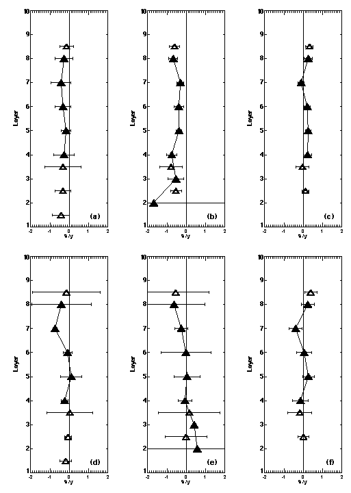
Figure 2.21 Hemispheric average regression slopes (%year-1) of the layer-ozone times series of coincident observations for the northern hemisphere in the top panels and for the southern hemisphere in the bottom panels. These averages result from the same stations used in Figure 2.19. All errors bars shown are ±2 standard errors of the mean (i.e., an estimate of the variance between stations). Panels (a) and (d) show the average slopes of the Umkehr observations; panels (b) and (e) show the average slopes of the SAGE I/II observations; and panels (c) and (f) show the variance-weighted average slopes ±95% confidence intervals associated with the variance-weighted means of the coincident-pair differences (Umkehr-SAGE within 2.5° latitude and 48 hours). The variance-weighted 95% confidence interval is calculated as 2 [(S s i -2) -1]1/2, where s i is the standard deviation of the regression slope of an individual station time series. The disconnected open triangles represent layers 1 through 10 plotted at layer 1.5; layers 2 through 10 plotted at layer 2.5; layers 2+3+4 plotted at layer 3.5; and layers 8+9+10 plotted at layer 8.5. The solid triangles represent individual layers. All Umkehr observations are individually corrected for aerosol interference by using the Mateer and DeLuisi aerosol correction factors.
The combination of Umkehr errors, SAGE II uncertainties, and atmospheric variability allows statistically significant information, at the 95% confidence level, to be obtained regarding the correspondence of Umkehr and SAGE I/II layer-ozone trends to within approximately 0.2%/year.
It is desirable to create a composite data set from SBUV and SBUV2 measurements so that a comparison can be made against the SAGE measured ozone trends in the upper stratosphere. There is a 17 month overlap between the two SBUV data sets beginning in January 1989. The percent differences between the two sets as a function of time for Umkehr layer 8 are illustrated in Figure 2.22 for three latitude bands. There are consistent offsets throughout most of 1989 but near the end of that year they begin to drift apart. Similar patterns are observed in other layers. Comparisons with Nimbus 7 TOMS total ozone measurements suggest that changes in the SBUV data are responsible for the change in behaviour. It is therefore recommended that the data for 1989 alone be used to determine an adjustment for the SBUV to SBUV2 transition of approximately 2% in layer 8 and by -4 to 4% in the other layers. Furthermore the 1990 SBUV data should be discarded.
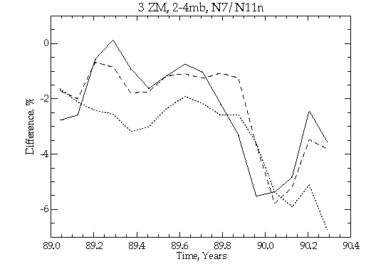
Figure 2.22 Time series of zonal/monthly mean differences (percent) between SBUV and SBUV2 for Umkehr layer 8. Solid line is for 30 ° N -50 ° N, the dashed line is for 30° S -50° S and the dotted line is 20° N to 20° N.
The mean differences between SAGE II and the coincident, adjusted SBUV2 from 1989 to 1994 are shown in Figure 2.23. The differences are just a few percent different from those between SAGE and SBUV measurements (see Figures 2.5 and 2.6 in section 2.3.2.1), but they show the same features, particularly in the latitudinal structure seen in layers 4 and 5. Of concern however is that the linear slopes of SBUV2 data from 1989 to 1994 are mostly larger than the linear slopes in SAGE data (shown in Figure 2.24). Although these slope differences are typically not significant individually at the 2 standard error level, there are obvious systematic differences in the global averages at levels 5 (+0.8 ±0.2%/year-1), 7 (+0.7 ±0.2%year-1), 8 (+1.3 ± 0.2%year-1) and 9 (+0.6 ±0.3%year-1).
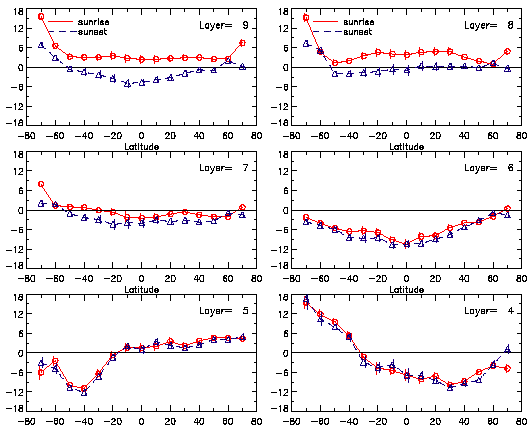
Figure 2.23 Mean percentage differences between SAGE II and coincident SBUV2 ozone values (SBUV2-SAGE) as a function of Umkehr layer and latitudinally binned in regions 10 wide. The error bars are twice the standard errors of the differences and SAGE sunrise and sunset measurements have been analysed separately.
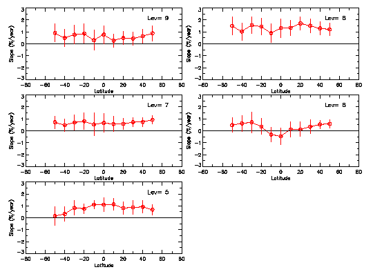
Figure 2.24 Mean slopes of SBUV2-SAGE coincident differences in Umkehr layers and in 10° latitude bins over the period of 1989-1994. Slopes are expressed as percent of the SAGE values per year. SAGE sunrise and sunset observations have been combined into a single time series.
These comparisons are based on the conversion of SAGE values to pressure surfaces which can cause changes in SAGE trends, whereas the other satellite instruments, such as SBUV2, intrinsically report ozone values on pressure surfaces. During the 1989 to 1994 period, geopotential height changes in the upper stratosphere (layers 7 to 9) could have produced anomalous trends of up to 1%/year in the tropics (see Section 2.2.2). However the effect would have been in the direction of increasing the SAGE ozone trends. It is concluded therefore that there must be other reasons for the larger slopes for SBUV2 than for SAGE.
It is to be noted that SBUV comparisons (see Chapter 1) show that SBUV2 may have had a calibration drift of approximately 0.5%year-1 at 1 hPa. Also the NOAA-11 satellite had changing equator-crossing times over time, and thus SBUV2 did not have a repeating pattern of solar zenith angles (SZA) from year to year as was the case for SBUV. These changing SZAs could have combined with interchannel calibration errors and modelling imprecision (e.g., in multiple scattering and temperature profiles) to create false changes in the profiles (see Chapter 1).
Despite these slope differences, the good overall quality of the two data sets may be seen in a comparison of the amplitudes of the annual cycles in the SAGE II and coincident SBUV2 measurements. These results are shown in Figure 2.7 (c) and (d) in section 2.3.2.1. As in the SAGE I/SBUV comparison the differences in the seasonal cycles are at the level of the uncertainties in the estimates (approximately 3%). There is remarkable similarity in the principal features of the two results but there is also possible evidence of a loss of vertical resolution in the SBUV2 observations at altitudes below 10 hPa. For example, the smaller maximum at 12 hPa in the southern hemisphere in the SBUV2 observations may be noted; however the SBUV observations for 1985-1989 (not shown) show a maximum similar to the SAGE II results in Figure 2.7 (c) in section 2.3.2.1.
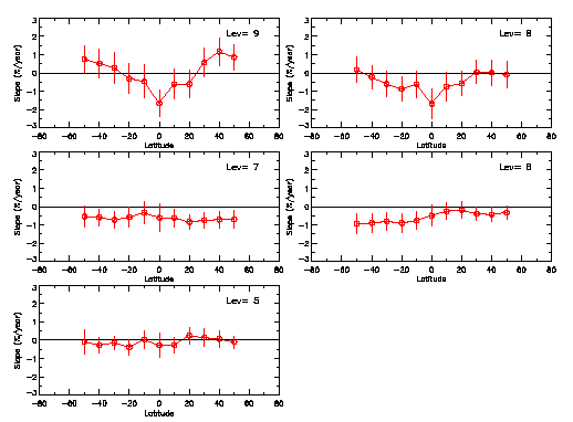
Figure 2.25 Mean slopes of SBUV-SAGE differences based on coincident SBUV measurements from 1984 to 1990. SAGE values have been summed over Umkehr layers and the differences have been accumulated in monthly bins which are 10 degree wide in latitude. Slopes are expressed as percentages of the SAGE mean values per year. SAGE sunrise and sunset differences have been combined.
Differences in the slopes calculated from SAGE II and coincident SBUV measurements from the end of 1984 to mid-1990 are shown in Figure 2.25. The differences are less systematic than for the SBUV2 comparisons, and in contrast to those results, they show that SAGE II exhibits more positive slopes than SBUV. The latitudinally averaged slope differences in layers 8-9 are approximately -0.2 ±0.4%year-1 (where the second term is the 2 standard error of the differences). The globally-averaged slope differences average -0.4 ±0.3%year-1 in layers 5 to 9. Again some of the tropical slope differences between SAGE II and SBUV in layers 8 and 9 in particular might be introduced by anomalous NWS temperature trends in the tropical upper stratosphere (and in contrast to the SBUV2 comparisons the possible errors are in the correct direction to explain the differences).
SBUV2 ozone profile retrievals are often given as 12 layer amounts. This does not mean that the instrument is capable of providing independent information for each of these layers. Since the SBUV2 ozone profile retrieval system is complex, it is difficult to determine whether trend results from other sources are consistent with SBUV2 results. However a study (Miller et al., 1997), based on perturbing SBUV profiles with simulated retrievals of ozone changes measured by SAGE and the sondes, shows that SBUV2 should provide accurate estimates of the ozone trends in layers 6-9 and in the sum of layers 1-5. Instead of layer 9 alone, it may also be better to use the sum of layers 9 to 12.
The eruptions of El Chichon in April 1982 and Pinatubo in June 1991 impacted the ability of SBUV and SBUV2 to make accurate measurements of ozone. The aerosol load injected into the lower stratosphere increased UV scattering and enhanced the backscatter signal. It is recommended that one year following both the Pinatubo and El Chichon eruptions SBUV data should be deleted from any time series for trend analysis. A more detailed characterisation of the relationship between the size and profile of these errors and the aerosol loading is presented in Torres and Bhartia (1995).
A comparison of the linear slopes in SAGE I and SBUV data is not meaningful because the period of operation of SAGE I was less than 3 years. A more useful slope comparison is obtained from the combined SAGE I/SAGE II data versus the coincident SBUV measurements. The slopes in the monthly mean differences are shown in Figure 2.26. SAGE data possess a more positive slope in layers 5 and 6 and a less positive slope in layers 8 and 9. The most significant difference is +0.4 ±0.2%year-1 in layer 9. However because of the offsetting differences in layers 5 to 7, it is concluded that overall there is no evidence of a drift in the SAGE (and overall SBUV) calibration of greater than 0.2%year-1, based on SBUV comparisons over the period 1979-1990. This is perhaps the longest period over which comparisons can be made between coincident ozone measurements obtained by essentially two separate instruments. It is likely to provide the strongest constraint possible on the absence of a drift in the SAGE ozone calibration.
In summary, SBUV comparisons for the 1984 to 1990 pre-Mt Pinatubo period validate the globally averaged SAGE II trends to within 0.4 ±0.3%year-1 with SAGE II showing a larger trend and they validate the globally averaged data for the longer record from 1979 to 1990 (i.e. including SAGE I data in the time series), to the 0.2%year-1 level for layers 5 to 9. Comparison of trends with SBUV2 show that SAGE II trends are smaller than SBUV2 by 0.8±0.3%year-1 and it is believed that the problem is caused by a solar zenith angle correction problem with the SBUV2 data.
Figure 2.26 Linear slopes of the differences (SBUV-SAGE) between SAGE and coincident SBUV ozone observations from 1979 to 1990 expressed as a percentage of the SAGE Umkehr layer. Mean values were binned by month and placed in 10 degree wide latitude bins. Error bars are twice the standard errors of the differences in slopes.
2.4.5.1. General Considerations
The SAGE II and HALOE (Russell et al., 1993) experiments are in identical 600 km, 57o inclination circular orbits. Because the orbital insertion times for these two experiments are different however, actual coincidences do not occur very often especially in the tropics because the ground tracks of the measurements sweep very rapidly through the region. In the range from 40° to 50° north or south, there are many more measurement coincidence opportunities because the measurement track is "turning around" in latitude and there is a tendency for the measurement location to "dwell" for some number of days before beginning another "rapid" pole-to-pole traversal. Three kinds of intercomparisons were performed; (1) absolute SAGE versus HALOE profile comparisons made at "coincident" points, done primarily to form an idea of the overall quality of the two data sets; (2) comparisons of annual changes in ozone obtained from linear fits to each of the two data sets; and (3) comparisons of changes in SAGE and HALOE differences with time obtained from spatially and temporally matched pairs of measurements from the two experiments. In addition to linear fits to the unmodified data sets, annual and semi-annual oscillations (AO and SAO) were also removed while doing the linear fits to assess possible improvements in agreement between the data sets.
2.4.5.2. Absolute Profile Differences
Statistical comparisons of SAGE II and HALOE profiles in the tropics and mid-latitudes were performed for the July/August periods of 1992 and 1996 respectively. These years cover times of peak Mt. Pinatubo aerosol loading and near background levels. The coincidence criteria used to select the SAGE II/HALOE pairs were 1 day, 2o latitude, and 12.5o longitude. SAGE II was used as the reference in computing percentage differences. The first point to note is that between 25 and 50 km, the two satellite results agree to within 5% or less. At lower altitudes, the differences are larger. In 1992, the SAGE II data do not extend below about 22 km due to effects of aerosol interference. Differences with HALOE at that level are large (~20%). In 1996 (when the aerosol loading is reduced) the SAGE II data extend down to lower altitudes and differences as large as 20% are not reached until about 18 km. All the reasons for differences in the two measurements below about 20 km are not known, but it is clear that aerosol effects in one or both experiments are a major cause for the discrepancies. This suggests that it will be difficult to draw meaningful conclusions about the validity of SAGE II long-term changes in the region below 20 km using SAGE II/HALOE comparisons. The SAGE II and HALOE differences are similar in sign and altitude dependence to the SAGE II versus ozonesonde differences shown in Section 2.4.1.
2.4.5.3. Long-Term Changes
The measurements from each experiment were prepared for long-term change comparisons by binning the data into 10o latitude intervals. Additionally for SAGE II, the data were filtered at altitudes below 25 km to remove any points with ozone errors greater than 12% to reduce possible aerosol effects on calculated long-term changes. The data in each latitude bin were then linearly interpolated to a 5 km altitude grid covering the altitude range from 15 km to 50 km. The ozone parameter analysed was number density. A least squares, linear fit was made to the entire SAGE II and HALOE data sets for the 1991-1996 and 1993-1996 time periods. These periods were selected to examine long-term change measurements during times when the Mount Pinatubo aerosol cloud was a maximum and when the effect was reduced. At each altitude, the linear change in percent per year was calculated using the middle point on the fitted line as the reference value. In the first set of comparisons, no attempt was made to remove natural cycles; we next removed the AO and SAO effects to assess how this would affect the results. In doing this, daily O3 values for a particular latitude bin were averaged longitudinally to get zonal means and fits were done to determine coefficients of mean, AO, SAO, and linear terms. There was a slight improvement (~0.5%year-1) in agreement with the natural cycles removed, so these data were used for the conclusions we draw.
Examples of the SAGE II and HALOE time series for the 30°-40°S bin are shown in Figure 2.27 for 20 km, 30 km, and 40 km altitude levels. Both time series show annual and semi-annual cycles at certain altitudes and the amplitudes of the variations are close in magnitude. At 20 km, clear differences between SAGE II and HALOE measurements exist in 1992, the year of peak aerosol loading. These general difference features exist for all latitude bins. Figure 2.28 shows the SAGE II and HALOE slopes as a function of latitude for each altitude level in 5 km increments for the 1991-1996 period with the AO and SAO removed. The error bars on the plots are the 2 standard error mean (sem) slope uncertainties. Note that down to 30 km, the differences in indicated annual changes are £ 0.5% at all latitudes except 55oS where they are ~1%. This is also true for 25 km at many latitudes, but there are two latitude bands, i.e. 15°N and 55°S, where the differences are 1.5% to 2%year-1. At 20 km, the differences are on the order of 2 to 4%year-1. A similar plot for the 1993-1996 period showed only small differences except at altitudes at and below ~25 km where there were slight improvements. The global mean differences in indicated annual changes for the 60°S to 60°N range are given in Table 2.7. The results show that from 50 km down to 25 km, while there are no statistically significant differences, the values are less than 0.2%year-1 at all altitudes except 30 km where it is 0.4% ± 0.25%year-1. At 20 km, the globally averaged differences are barely significant at the 1.4% ± 1.2%year-1 level. Below 20 km, the differences are large and no useful results are obtained in the tropics because of poor sampling.
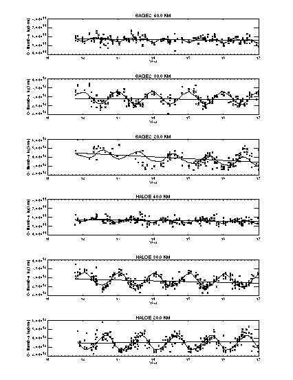
Figure 2.27 SAGE II and HALOE time series for the UARS period in the 30oS-40oS region for the 20 km, 30 km, and 40 km altitude levels. Annual, semi-annual, and linear fits are shown.

Figure 2.28 SAGE II and HALOE linear trends versus latitude for the 15 km to 50 km altitude range. Annual and semi-annual oscillations were removed while performing the linear fit.
|
Altitude
|
Difference |
2 Standard
|
|
|
|
|
|
|
|
|
|
|
|
|
|
|
|
|
|
|
|
|
|
|
|
|
|
|
|
|
Table 2.7: Global Mean (60oS-60oN) Difference (HALOE -SAGE II) in Indicated Annual Ozone Change in units of %year-1.
2.4.5.4. Changes in SAGE II/HALOE Differences
The next comparison performed was to calculate differences in SAGE II and HALOE data "co-located" in time and space. The main purpose of this comparison was to examine the data to see if there was any time dependence of the differences, either seasonal or longer term, which would imply an instrumental or experiment effect that may be giving rise to false trends. In each latitude bin, profiles from the two experiments were matched using coincidence criteria mentioned above. Each data set was interpolated to a 1 km altitude grid and percent differences were calculated using the average of SAGE II and HALOE as a reference.
The percent difference values were then interpolated to the standard 5 km altitude grid used in this report. One problem with this approach is that the number of data points used for calculating long-term changes dramatically reduces when a matching criterion is applied; so much so in the tropics, that meaningful comparisons cannot be made. The latitude range with the most coincidences is 30°-40°N or S. A marginal number of coincidences exist at 20 km and there are not enough at 15 km to use in this study. There appears to be a slight seasonal dependence of the differences but without other corroborating data (which has not been borne out in this study), no conclusions can be drawn. Over the 25 km to 50 km range, the only latitude ranges where there are consistent statistically significant slopes to the difference time series are 400-50oS (~1.5%± 1%year-1) and 60o-70oS (0.5± 0.5%year-1). Below 25 km, the differences are not statistically significant. In each latitude bin, the change is negative, i.e. SAGE II appears to be getting progressively larger with time than HALOE or vice versa. When viewed globally, i.e. when the same analysis is done on a single time series of HALOE-SAGE II differences using the entire 60°N-60°S range, the results are very similar to those shown in Table 2.7.
2.4.5.5. Summary and Conclusions
Comparisons of annual changes determined from simultaneous annual, semi-annual, and linear fits to the full SAGE II and HALOE data sets over the 1991-1996 time period show agreement in the 50 km to 30 km interval to better than ± 0.5%year-1 at all latitudes except 55oS where they are ~ 1%year-1. Agreement to £ ± 0.5%year-1 is also obtained for 25 km at all latitudes except 15°N and 55°S where they are 1.5% to 2%year-1. If the AO and SAO effects are not included in the fit, the agreement degrades by about 0.5%year-1. This suggests that sampling differences between the two experiments may be falsely indicating long-term change. The globally averaged mean differences in annual change from 50 km down to 25 km are 0.2± 0.2% -0.6%year?1 (-0.4 ± 0.3%year?1 at 30 km). Using matched SAGE II/HALOE pairs, plotting percent differences versus time, and then doing a linear fit through the difference points shows no statistically significant SAGE II drifts with time relative to HALOE over the 50 km to 25 km interval except at 40o-50oS (~1.5± 1%year-1)and 60o-70oS (~0.5± 0.5%year-1). No statistically significant drifts are observed at any other latitudes. On a global basis, the averaged "trends" of the HALOE-SAGE II difference time series at various altitudes show similar results as those obtained using non-coincident data. Because of the large differences in annual change observed below 25 km between SAGE II and HALOE and without knowing the cause of the differences, no conclusions can be drawn regarding the validity of SAGE II data for trend calculations in this region.
2.4.6.1. Introduction
The concept of employing dynamical techniques for the intercomparison of sparse data sets was introduced in Section 2.2.5. Here the Coordinate Mapping (CM) technique is used to compare the UARS-period mean ozone values and simple linear trends in SAGE and HALOE observations. Section 2.4.6.2 describes the technique and discusses the advantages and disadvantages of its use as a data intercomparison tool. In Section 2.4.6.3 the effectiveness of the CM technique is verified through comparison with the more conventional zonal mean approach for a test period in March 1995, during which SAGE and HALOE made observations at similar latitudes. Results of the CM analysis for the UARS period are reported in Section 2.4.6.4. Finally, Section 2.4.6.5 introduces the Trajectory Mapping (TM) technique, a second dynamical approach to data intercomparisons which has promising potential for future work.
2.4.6.2. Coordinate Mapping
The general concept of employing quasi-conservative coordinate mapping as a means of increasing the utility of available stratospheric trace gas data dates back to McIntyre (1980), who referred to it as a "modified Lagrangian mean" approach to stratospheric analysis. The method, formally developed by Schoeberl and Lait (1993), has been utilized in recent years as a powerful tool with numerous applications (e.g., Lait et al. 1990; Randel and Wu, 1995; Atkinson and Plumb, 1997), including the intercomparison of sparse data sets at high latitudes, where the ozone field tends to be most variable (Redaelli et al., 1994). The technique involves a transformation of trace gas data from 3-D physical space (latitude-longitude-pressure) into 2-D potential vorticity (PV) ? potential temperature (PT) coordinates, a flow-following "dynamical" reference frame. The 2-D character of this reference frame makes it analogous to a zonal mean analysis. However, because the dynamical coordinates move with the meteorology when the flow is adiabatic, it is possible in this reference frame to reduce the contribution to "local" variance in ozone concentrations due to short-period meteorological variability. Also, since the instantaneous large-scale stratospheric wind field is typically closely aligned along isopleths of isentropic PV, ozone mixing tends to be very rapid along a PV contour as compared to mixing across it. The isentropic ozone mixing ratio contours therefore closely mimic those of the PV [Leovy et al., 1985; Butchart and Remsberg, 1986; Manney et al., 1995], so that over suitably short periods (compared to photochemical and diabatic time-scales), "longitudinal" and temporal variations in this dynamical reference frame will be small. Therefore, comparing sparse data sets in this coordinate system should reduce biases introduced by the different time and spatial sampling of the individual instruments. The reliability of the CM results is dependent upon the quality of the meteorological analyses, and the extent to which the PV, PT, and ozone mixing ratio are conserved along the flow. The validity of these assumptions varies as a function of latitude, altitude, and season, but these assumptions generally hold true in the lower stratosphere. Overall, the technique is a computationally inexpensive and efficient means of comparing sparse data sets.
2.4.6.3. Technique Verification
To gauge the reduction in variance possible through use of dynamical techniques, we calculate the standard deviation of March 1995 SAGE observations in 5 degree latitude bins on altitude surfaces (traditional approach) and 5 degree equivalent latitude (Butchart and Remsberg, 1986; Lary et al., 1995) bins on potential temperature surfaces. Equivalent latitude is a form of normalised PV closely associated with geographical latitude. In regions where the flow is zonally symmetric, or the dynamical time-scale is much longer than chemical or radiative time-scales, equivalent latitude reduces to geographical latitude. The standard deviations of the observations showed general patterns across broad latitude bands, and were thus averaged into broader bands. Figure 2.29 shows the results for (a) 30-50oS, (b) 50-65 oS, (c) 30°-50°N and (d) 50°-70°N. In regions where the photochemical and dynamical time scales are long, such as at high latitudes in both hemispheres (panels b and d) and at northern mid-latitudes (panel c) in the lower stratosphere, CM shows a reduction in variance as compared to the traditional approach. In the tropics (not shown) and southern mid-latitudes (panel a), where the flow is less disturbed or photochemical time scales are short (i.e. in the tropical upper stratosphere), the CM results are consistent with traditional results. The period March 19-21, 1995 was selected to assess the effectiveness of the CM technique. During this 3-day period, HALOE and SAGE were observing at the same latitudes in both hemispheres. As a result, the traditional zonal mean approach should have produced its most reliable results. First, zonal means of SAGE and HALOE profiles meeting standard coincidence criteria were created, similar to the analysis in section 2.4.5.2. Then SAGE and HALOE observations for March 6-31 were mapped into dynamical coordinates using the CM technique. Using the National Centers for Environmental Prediction (NCEP) global analyses interpolated to the satellite measurement sites, we interpolated HALOE and SAGE ozone data for this period onto PT surfaces and separated the data into bins of 2 PV units (1 PVU = 3 x 10⁻⁶ K m2 kg-1 s-1) on each level. Measurements in each bin were averaged to define a composite field in PV ? PT space for each instrument, using data collected for periods of ± 10 days (21 days total). Composite fields were constructed on March 16 and 21, and in-between days were linearly interpolated. SAGE data with corresponding quality flags in excess of 12% of the observation values were excluded. To compare with the traditional results, the HALOE and SAGE measurements were then mapped back into physical space. Using the 12Z March 20 NCEP dynamical data and the PV-PT composite fields, we reconstructed synoptic SAGE and HALOE measurements at the resolution of the dynamical data (2 degrees latitude by 5 degrees longitude). Finally, we calculated the zonal mean of the CM coincident measurements.
Figures 2.30a shows the percent difference between SAGE and HALOE standard zonal mean ozone profiles in the northern (64°-66°N) and southern (29°-35°S) Hemispheres. The error bars represent the 2s standard error in the zonal mean calculation. The agreement between the two data sets is within 5% in the northern hemisphere, with no statistically significant differences. Larger differences exist in the southern hemisphere below 22 km, with HALOE ozone generally lower than SAGE ozone. These differences may be due to the presence of aerosols. Figure 2.30b shows the percent difference between zonal mean CM HALOE and CM SAGE ozone measurements as a function of height at 65°N and 30°-34°S. The agreement between these zonal mean difference profiles is within 5% of the traditional results in both hemispheres. The CM technique indicates greater statistical significance in the northern hemisphere lower stratosphere, where the technique should be performing well (see Figure 2.29d). This demonstrates the validity of the technique as compared to the traditional approach during a time period when the traditional approach is performing its best. This is true in both hemispheres, despite the reduced variability in the southern mid-latitudes (see Figure 2.29a). Further, small errors introduced by meteorological uncertainties, for example, should be random, and thus not contribute to trend uncertainties. The CM technique gives results consistent with traditional comparisons, but, unlike the traditional approach, CM can comment on the agreement between SAGE and HALOE at latitudes and during time periods outside of those when SAGE and HALOE are coincidentally observing the same latitudes.
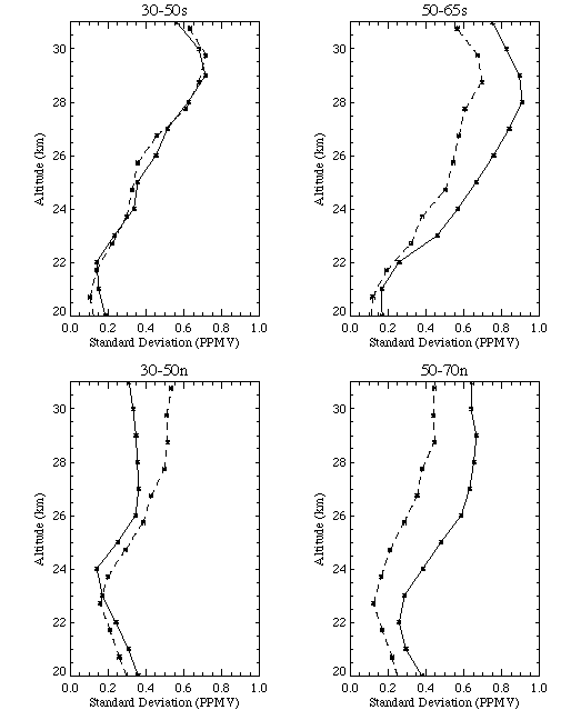
Figure 2.29 Standard deviation of March 1995 SAGE observations in 5 degree latitude bins on altitude surfaces (traditional approach) and in 5 degree equivalent latitude bands on potential temperature surfaces (Lagrangian-mean approach). Plotted are average standard deviations at (a) 30oS-50oS; (b) 50 oS-65oS; (c) 30oN-50oN; and (d) 50oN-70oN in each coordinate system.
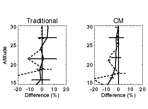
Figure 2.30 March 19-21, 1995 (HALOE-SAGE)/SAGE ozone percent difference profiles at 64°N-66°N (solid line) and 29°S-35°S (dashed line) for (a) Traditional results and (b) Coordinate Mapping results. Traditional results are coincident-matched profile differences calculated on pressure surfaces. CM results are percentage differences between CM HALOE and CM SAGE calculated on potential temperature surfaces for 65°N (solid line) and 30°S-34°S (dashed line).
2.4.6.4. Coordinate Mapping-Based Intercomparison of SAGE II with HALOE
2.4.6.4.1. Analysis Technique
Each SAGE and HALOE profile from 20 September 1991 to 31 December 1996 was first interpolated to 24 isentropic levels from 300K and 1200K. Daily NCEP stratospheric analyses were then used to transform the data at each level from geographic into equivalent latitude. Finally, a 2-D gaussian interpolation scheme was used to produce 5 degree equivalent latitude by 1 month ozone fields for each instrument. The individual measurements were weighted by the distance from the grid point and by the reported measurement error. This weighting was used to eliminate spurious extrapolated values from consideration. At each isentropic level and equivalent latitude, UARS period mean and seasonal differences and simple least-squares trends in the differences were calculated. The latter quantity should be indicative of UARS period mean drift between SAGE and HALOE.
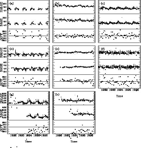
Figure 2.31 UARS period time series of raw and analysed ozone mixing ratio for HALOE, SAGE, and their percentage differences at a range of equivalent latitudes and potential temperatures. (a) 76°S at 1100K, (b) 4°S at 1000K, (c) 60°N at 1000K, (d) 64°S at 650K, (e) Equator at 650K, (f) 40°N at 700K, (g) 60°S at 400K, and (h) 4°S at 475K. Crosses denote raw observations made within 2 degrees equivalent latitude of the central latitude, and open squares the monthly gridded values. Filled squares are the monthly percentage differences.
2.4.6.4.2 Results
Figure 2.31 shows a selection of UARS-period time series of the data from SAGE and HALOE, and their percentage differences, for selected values of potential temperature and equivalent latitude. This figure demonstrates the degree of effectiveness of the analysis technique in describing the "modified Lagrangian mean" ozone evolution observed by each instrument during the period. The seasonal data gaps evident in Figures 2.31a and d, for the high southern latitudes, suggest that any results for this region are likely to be seasonally biased. Figures 2.31e, g, and h reveal the very limited record available for the calculation of trends in the lower stratosphere.
Figure 2.32 shows the period mean percentage difference (HALOE-SAGE) between SAGE and HALOE observations. In general, SAGE sees considerably more ozone than HALOE throughout the lower stratosphere, more so with decreasing altitude (see Figures 2.31g and h). This is consistent with the sonde results reported in section 2.4.1. Above about 600K (~25 km) SAGE and HALOE typically agree to within a few percent, though larger differences are present in the mid- to high latitude upper stratosphere and the tropical middle stratosphere (around 700K) where HALOE ozone exceeds SAGE by 2%. In the mid-latitude middle stratosphere, SAGE exceeds HALOE by 2.5%. An examination of the seasonal variations in the differences (not shown) indicates that the upper stratospheric differences are largely a summer feature (see Figure 2.31a and c). Figure 2.31e suggests that HALOE may see a stronger QBO cycle in ozone than SAGE in the tropical middle stratosphere below the ozone maximum.
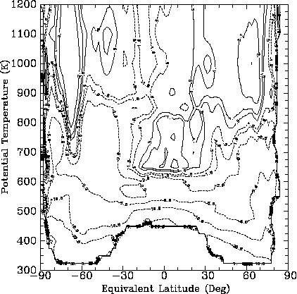
Figure 2.32 UARS period mean, modified Lagrangian mean cross-section (equivalent latitude versus potential temperature) of percentage difference between HALOE and SAGE ozone mixing ratio (i.e. 100*(HALOE-SAGE)/SAGE).
Simple least squares linear trends were calculated for each instrument and for the differences between the two instruments. The relative drift between instruments is shown as a function of equivalent latitude at 4 PT levels in Figure 2.33. At 650K (~25km) HALOE observations at most latitudes in the middle stratosphere tend to have drifted downward relative to SAGE, by up to a percent or so per year. This is where, according to Figure 2.32 period mean HALOE ozone is lower than SAGE, suggesting the gap between the two instruments has widened during the UARS period. The CM analysis shows three regions of statistically significant drift between the instruments at this level. At southern high latitudes, the results are in good agreement with traditional comparisons (section 2.4.5) showing negative HALOE drift relative to SAGE of 1-2%/year from 45o-60oS. The CM results are also consistent with a HALOE negative drift of 0.5%/year at 60o-70oS (section 2.4.5), keeping in mind that the drift in this latitude range maps to the average drift in the equivalent latitude range of ~60o-90oS. In this case the individual instrument analyses (not shown) show a statistically significant decrease in HALOE ozone, while SAGE shows an insignificant increase over the same period. The positive HALOE relative drift in the southern subtropics of ~ 2± 1%/year is consistent with results shown in Figure 2.28 in Section 2.4.5.3. However, the significant negative HALOE drift at the equator is most likely a consequence of the two extraneous data points at the end of the HALOE time series, as seen in Figure 2.31e. In the 40°-50°N equivalent latitude range, the CM analysis indicates a negative drift of HALOE with respect to SAGE of ~1± 0.75%/year. In this region the trend in SAGE observations is near zero, while the HALOE data show an ozone decrease on the order of 1-1.5%/year. A similar tendency can be seen in the trend comparisons in Figure 2.28 in Section 2.4.5.3.
Above 800K (~30 km) the CM analysis suggests that the mean drift between SAGE and HALOE is generally small (less than 0.5%/year) and not significant, except at polar latitudes. In the northern polar regions at 800K and 1000K (~ 36 km), summertime HALOE observations have drifted downward significantly with respect to SAGE (~ 3-4% ± 3%/year) with SAGE during the period showing ozone increases not detected by HALOE. A similar feature is present in the southern hemisphere at 1200K (~ 40 km) as also seen in Figure 2.31a. The two instruments agree on a significant downward drift in tropical upper stratospheric ozone (above 750K) of up to 2%/year during the period (see Figure 2.31b). This is consistent with the findings using traditional techniques shown in Figure 2.28 at 35 and 40 km (see Section 2.4.5.3). In the lower stratosphere (not shown), the short record length considered makes it meaningless to interpret more than the period mean differences. Of note in Figure 2.31g, though, and to a lesser extent in Figure 2.31h, is an indication that the drifts derived for these locations may be unduly influenced by aerosol-affected observations from the Pinatubo period which have escaped rejection by the data quality filter.
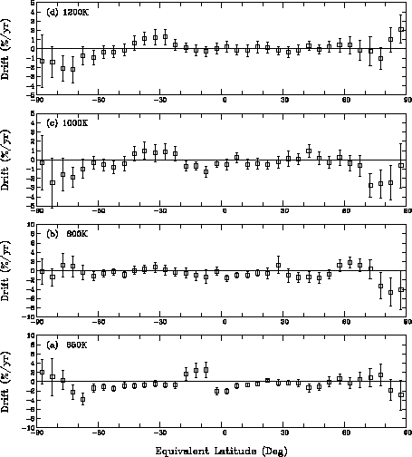
Figure 2.33 UARS period drift between monthly analysed SAGE and HALOE ozone (%/year) as a function of equivalent latitude at (a) 1200K (~ 40km); (b) 1000K (~ 36km); (c) 800K (~ 30 km); (d) 650K (~ 25 km). Error bars are 95% confidence limits.
2.4.6.5. Trajectory Mapping
Trajectory mapping (TM) is another dynamical technique useful for the intercomparison of sparse data sets. Whereas the CM approach has its equivalent in the intercomparison of monthly zonal mean data, the TM technique is the "dynamical" equivalent of the traditional coincidence approach. Like CM, it takes advantage of quasi-conserved quantities following the motion, namely the ozone mixing ratio and potential temperature. Morris et al. (1995) noted that the latter of these is reasonably well conserved for about 7 to 10 days.
To create a synoptic trajectory map from satellite data, air parcels are initialised in the model at the time and location of each satellite observation. These air parcels are then isentropically advected forward or backward in time by the model using analysed wind fields. Because trajectory maps include observations from a number of days, they yield substantially enhanced coverage compared to asynoptic maps produced from a single day of measurements. Furthermore, by correctly accounting for dynamical changes in the atmosphere between observations, TM, like CM, provides better representations of the measured constituent fields than asynoptic schemes. Trajectory mapping can be straightforwardly applied to data intercomparison, as shown in Pierce et al. (1994a and b), Morris (1994), Morris et al. (1995) and Morris et al. (1997). By creating trajectory maps of observations from one instrument at the time of the observations of a second instrument, individual pairs of observations (which may have been made at widely different locations and times) can closely coincide and be directly compared. Frequently, these pairs would have failed the coincidence criteria used in the traditional approach and would therefore have been eliminated from consideration. The main disadvantages of the TM technique are the need for accurate global wind velocity fields (like the CM approach) and the high computational cost (unlike CM) which makes the technique impractical for intercomparisons over decadal time-scales.
The use of TM techniques in satellite data validation is summarised in Morris et al. (1995) and Morris et al. (submitted 1997; Web: ftp:/hyperion.gsfc.nasa.gov/pub/papers/morris/jgr.paper4). Morris et al. (1997) presents results using the TM analysis for the same March 1995 test period as above. Figure 2.34 shows a scatter plot of (a) the coincident ozone measurements retrieved by HALOE and (b) 3-day, trajectory-mapped HALOE averages versus SAGE observations at the 800 K level. Using a 400 km and 12 hours coincidence criteria gives 120 coincidences (a stricter time criterion of 10 hours results in fewer than 10 coincidences), or ~20% of the total measurements made by HALOE and SAGE during this time period. Furthermore, the coincident approach can only comment on the relationship between the two instruments in the restricted latitude bands of concurrent observation (e.g., 64°?66°N, 29°?35°S). Using the TM technique, the number of coincidences increases from 120 to 202. More coincidences occur with longer trajectory calculations, but this improvement is balanced by the increased uncertainty with longer trajectories. At 800K, the RMS difference is 10.0% for the traditional coincidences compared to 7.1% for the TM pairs. In this study, trajectory advection periods of up to 7 days duration produced RMS differences in measurements which were smaller than those found using the traditional coincident comparison technique at all altitudes in the 64°-66°N range. The reason for this behaviour can probably be attributed to the method’s ability to reduce spatial and temporal variability.
2.4.6.6. Discussion and Implications
Both CM and TM techniques are effective methods for comparing "sparse" data sets. They increase the number and spatial extent of observations from each instrument that can be intercompared. This analysis and results from Morris et al. (1997) suggests the TM approach is more accurate than the CM technique, but it is also much more computationally expensive. As a result, TM is probably better used in closely examining particular pairs of observations, whereas the computational efficiency of the CM approach makes it ideally suited for intercomparing data sets over extended periods. The results obtained for the SAGE/HALOE intercomparison using the CM technique generally support those obtained using the classical "zonal mean" approach, but tend to be more significant. The CM intercomparison has also provided insight into instrument performance in regions of the atmosphere where data sparsity inhibits intercomparison by the classical coincidence techniques, and where "difference in trend" analyses likely suffer uncertainties due to the differential instrument sampling in space and time.
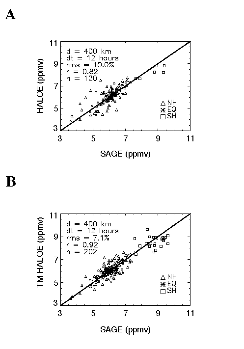
Figure 2.34 (a) HALOE vs. SAGE ozone using traditional coincidence criteria of 400 km maximum separation and 12 hour maximum time difference for the period March 12 - April 5, 1995 at the 800 K potential temperature surface (~10 hPa or 30 km). (b) HALOE vs. SAGE ozone on the 800 K (~30 km) potential temperature surface using the trajectory mapping approach. Trajectory calculations are limited to 3 days duration. Advected HALOE measurements within 400 km of the SAGE observations are considered coincident.
Two important qualifications should be made regarding the CM drift results. First, they are based on just five years of data, at most: whether or not the analysed drifts between the two instruments, for example, are representative of instrument behaviour over longer time scales, has not been addressed here. Second, erroneous temperature drifts in either the NCEP stratospheric analyses or the HALOE temperature retrievals could have a significant impact on this analysis. At these altitudes, both SAGE and HALOE ozone retrievals are based on first guess temperature and pressure profiles interpolated from the NCEP analyses, whereas HALOE retrieves its own temperature and pressure profiles above 30 km but uses NCEP data below. The first step in the CM-based analysis was the interpolation of all ozone profiles to isentropic levels. For this, the temperature profiles provided by the respective instrument team with each ozone profile were used (NCEP for SAGE, HALOE for HALOE), so any overall drift between HALOE and NCEP temperatures would induce an isentropic ozone trend wherever there is a vertical gradient in ozone. Perhaps as important, erroneous trends in the NCEP analyses could directly impact the SAGE retrievals through the pressure dependence of Rayleigh scattering in the SAGE ozone retrieval. On the other hand, real temperature trends depicted by both NCEP and HALOE should not influence the results presented here.
The CM analysis reveals ~ 0.5% differences in drifts above 30 km in all except the polar regions. At ~25 km the results show significant negative drift of HALOE with respect to SAGE at southern mid-high latitudes and to a lesser extent in northern mid-latitudes. The results also indicate a positive drift of HALOE relative to SAGE in the southern sub-tropics, which may be a manifestation of QBO differences in the data. These results generally agree with the conventional comparisons described in Section 2.4.5. The conclusion that no confidence can be placed in differences in differences in trends below about 22 km also agrees with the conventional analysis results. The analysis for the lower stratosphere suggests care should be exercised in interpreting trends based on data that include aerosol-affected measurements. Given the documented sensitivity of SAGE ozone retrievals to stratospheric aerosol, this analysis suggests, in support of the classical analyses, that it may be advisable to time-filter, rather than quality-filter SAGE data.
Comparisons have been made between SAGE II and coincident MLS measurements by averaging SAGE ozone measurements over UARS pressure levels. Occasional spikes found in the MLS data were found to be correlated with high values of the MLS ozone error bars. These spikes have been removed from the comparisons. Mean differences between SAGE II and MLS (version 4) are shown in Figure 2.35(a) to (c). MLS observations are retrieved with a vertical resolution of two UARS layers (~5 km). Comparisons between SAGE II and MLS will therefore emphasise 4.6, 2.2 and 1.0 hPa (and corresponding levels which differ by a factor of ten in pressure). MLS observations may be seen to yield a few percent larger ozone concentrations from 2.2 to 22 hPa. At 1.0 hPa MLS measurements are smaller than SAGE II values. This has been noted for some time (e.g. Cunnold et al., 1996b) but perhaps more remarkable is the apparent difference between the SAGE sunrise and sunset measurements of approximately 10% at 1 hPa. This difference is slightly larger than for SAGE version 5.93 results (see Figure 2.2 in Section 2.3.1). Fortunately at levels other than 1 hPa, the SAGE II sunrise/sunset differences are less than 5%, including in Umkehr layer 9 (see Figures 2.23 in Section 2.4.4. and 2.6 in Section 2.3.3.1 for example).
At 46 hPa SAGE II ozone values are larger than MLS values. This suggests that MLS values are too small at this level, particularly in the tropics; evidence for this has been previously discussed by Froidevaux et al (1996). However ozonesonde comparisons also suggest that SAGE II values are approximately 5% to 10% too large between 15 and 20 km altitudes (see Section 2.4.1); this may be contributing to the SAGE/MLS differences. At the 100 hPa level it is clear, and from other comparisons also, that the MLS values are substantially too large; there are known difficulties with the MLS retrievals at this level. Accordingly, trends at 100 hPa are not included in the comparisons of this section.
The relationship between SAGE II and HALOE ozone measurements can be examined by using MLS as a transfer standard (since there are only a smaller number of coincidences between SAGE II and HALOE measurements). Comparisons between HALOE (version 18) and MLS measurements (Figure 2.35(d) to (f)) show that HALOE values are also a few percent less than MLS values from 2.2 to 22 hPa. They confirm that MLS values are relatively smaller at 1 hPa (by approximately 5%) and they show a similar structure to the MLS/SAGE differences at 46 and 100 hPa, thereby also suggesting deficiencies in the MLS profiles at these two levels.
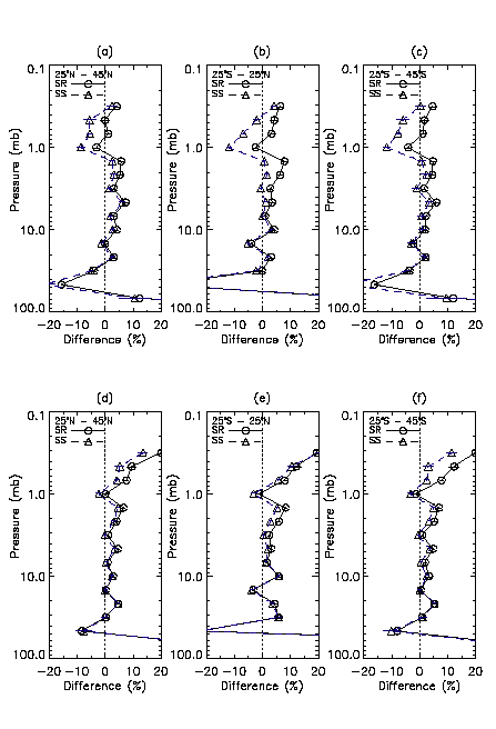
Figure 2.35 Differences (MLS-SAGE II) between (a), (b) and (c) SAGE II and (d), (e) and (f) HALOE (version 18) and coincident MLS (version 4) night time ozone measurements expressed as percentages of the MLS values. SAGE and HALOE sunrises and sunsets have been treated separately and the data were placed in three separate bins which extended from 25° S-45° S, 25° S-25° N and 25° N -45° N. The SAGE data were placed on pressure levels using the NWS temperature profiles and then summed over UARS layers which have boundaries at 103-I/6 hPa. The error bars are twice the standard errors of the differences. The period of comparison was October 1991 to December 1996 but the SAGE data has been filtered as recommended to remove the Pinatubo aerosol interference effects.
Since the 15-20 km altitude range is so important for this report, it is highly desirable to compare SAGE and HALOE at 68 and 100 hPa. Unfortunately the MLS observations are not sufficiently accurate at these levels that MLS data can be used as a transfer standard. Therefore a direct comparison of the mean SAGE and HALOE values over similar periods is shown in Figure 2.36. Differences are between ±2% at altitudes above 32 hPa but SAGE values are larger than HALOE values at altitudes below this particularly in the tropics. At 46 hPa similar differences are derived by using MLS as a transfer standard. At mid-latitudes below 20 km altitude (50 hPa) a hemispheric asymmetry of the differences (of approximately 5%) is also shown. This asymmetry is also present if pre-Pinatubo SAGE II data are projected forward in time using a time series fit to SAGE I/SAGE II trends. The low altitude differences might be related to altitude registration problems for SAGE II below 20 km altitude but the latitudinal asymmetry suggests that the effects may not be systematic and that SAGE II trends below 20 km altitude might be affected.
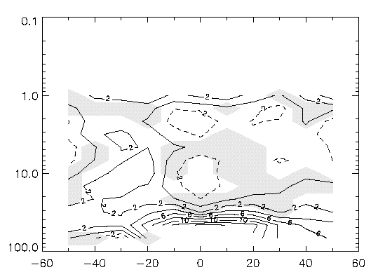
Figure 2.36 Mean differences between SAGE and HALOE measurements in percent determined from linear fits to SAGE and HALOE monthly means in UARS layers (but including annual and semi-annual cycles). The time series extended from October 1991 to December 1996 but started later at altitudes below 30 km where SAGE II data were filtered, as recommended, in order to remove the effects of aerosol interference.
Figure 2.37 shows a comparison of MLS and HALOE annual cycles in ozone. These may be compared against the SAGE II values which were compared earlier against the SBUV2 values (Figure 2.7 in section 2.3.2.1). In the lower stratosphere there are differences which reach 6% where the annual cycles are large and are changing rapidly with height. This is additional evidence that there are significant differences between the various measurements below 20 km altitude. Elsewhere however the results provide confirmation of the excellent quality of all three measurement systems.
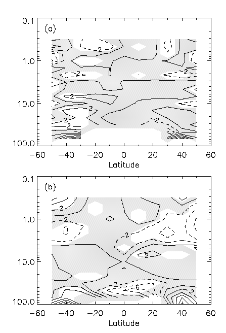
Figure 2.37 A comparison between the amplitudes of the annual cycles in zonal mean ozone expressed as percentages of the annual mean values from (a) HALOE and (b) coincident MLS observations. The HALOE measurements have been summed over individual UARS layers and data from October 1991 to December 1996 were used.
Linear slope differences from coincident SAGE II and MLS observations are shown in Figure 2.38. The overlap period is less than 6 years (and is only half this at altitudes below 40 hPa because of the prescribed filtering of SAGE II data). SAGE II slopes equal or exceed MLS slopes in the latitudinal mean at all levels from 1 to 46 hPa but there is no recognisable pattern in the differences and only at 22 hPa is the difference barely significant at the 95% confidence level. The mean of the slope differences between 1 and 46 hPa is -0.4 ±0.8%/year. As before, SAGE ozone slopes may be related to HALOE ozone slopes based on a comparison of slopes in coincident HALOE and MLS measurements. This comparison is also shown in 2.38. In this case, differences at 46 hPa seem to be related to an MLS problem during the first year after the Pinatubo eruption during which MLS ozone values, in the tropics particularly, exhibited a strong upward trend at 46 hPa which was not captured by the ozonesondes (Froidevaux et al., 1996) (the SAGE/MLS comparisons did not contain this period at these levels because of Pinatubo effects on SAGE II). The only significant MLS/HALOE slope difference at the 95% confidence level between 1 and 22 hPa occurs at 22 hPa where the HALOE slope is 0.9%year-1 less than the MLS slope. The differences in the 1 to 22 hPa region are latitude and altitude dependent and average -0.1 ±0.8%year-1.
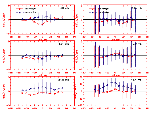
Figure 2.38 The slopes in the differences between coincident night-time MLS ozone observations from 1991 to 1996 and SAGE II (full line with circles) and HALOE (dashed line with triangles). The SAGE II data has been summed over UARS layers and filtered by the recommended procedure following the Pinatubo eruption. The error bars are twice the standard error of the slope estimates.
It is concluded that HALOE, MLS and SAGE II do not drift relative to each other by more than 0.5%year-1, which is within the measurement uncertainties. However all three sets of measurements yield significantly different slopes at 22 hPa with SAGE II yielding the most positive slope and HALOE showing 1.6%year-1. These differences are almost independent of latitude.
The SAGE II sunrise/sunset differences shown in Figure 2.35 (a)-(c) combined with the absence of sunrise/sunset differences in SAGE I observations suggest that there are long-term trend differences in the upper stratosphere between the sunrise and sunset results in the SAGE I/II record. These trend differences are shown in Figure 2.39. Similar differences between the two SAGE II alone trends are calculated if SAGE I observations are not used; furthermore comparisons against the SBUV measurements suggest that only approximately 0.1%year-1 of the differences can be attributed to sampling differences. The SAGE II comparisons against HALOE and SBUV measurements do not suggest a preference for sunrise or sunset observations. Furthermore Wang et al. (1996) noted the occasional presence of large differences of opposite sign between SAGE II sunset and sunrise observations at the same latitude when comparing against SBUV measurements (e.g. in January 1987). Thus SAGE trends are reported from the combination of sunrise and sunset observations and one-half the differences shown in Figure 2.39 are included in the reported (2) error bars.
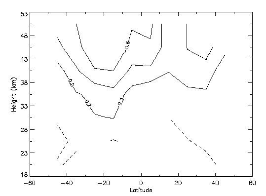
Figure 2.39 The difference between SAGE I/II sunrise and sunset trends from 1979 to 1996 (percent/year). The dashed lines are contours of zero percent/year and the latitude bins were 10 degrees wide.
Although intercomparisons which extend over relative short periods are not useful for evaluating the accuracy of long term ozone profile trends, they can be very valuable for assessing the relative accuracy and precision of the different instruments as a function of altitude. This section reports on results of a series of short term intercomparisons made during the last decade. First, SAGE II data are compared with observations obtained during the Atmospheric Trace Molecule Spectroscopy (ATMOS) experiment deployed on the Space-Lab-3 mission in April/May 1985 and the ATLAS-3 Space Shuttle mission in November 1994. Also, within the frame of the Network for the Detection of Stratospheric Change (NDSC) dedicated short term campaigns were conducted to compare multiple instruments that measure the stratospheric ozone vertical distribution. The results of three NDSC intercomparison campaigns are evaluated: STOIC (Stratospheric Ozone Intercomparison Campaign), OPAL (Ozone Profiler Assessment at Lauder) in April 1995 and MLO3 (Mauna Loa Ozone). Finally, time series of microwave observations made at Table Mountain and at Lauder were compared with SAGE II.
ATMOS/SAGE II comparisons:
For the most recent flight of ATMOS, that on ATLAS-3 [Gunson et al., 1996], there were 16 SAGE II sunset coincidences between 45°-54°N and 32 sunrise coincidences between 65°-74°S. In this particular comparison, both sensors recorded sunset occultations in the northern hemisphere and sunrise occultations in the southern hemisphere. The average ATMOS latitudes were 47.7°N and 71.4°S for sunset and sunrise occultations, respectively. The corresponding average SAGE latitudes were 51.5°N and 68.3°S, respectively. Sunset coincident days cover Nov. 4-6 for ATMOS and Nov. 3-7 for SAGE. Sunrise coincident days cover Nov. 7-11 for ATMOS and Nov. 6-12 for SAGE. The coincidence criteria are 5 degrees latitude, 1000 km distance, and 24 hours. Figure 2.40 shows the average ATMOS-SAGE percent difference for the 1994 flight for the sunset profiles in the upper left panel and for all the sunrise profiles in the lower left panel. The results of both sunrise and sunset comparison are similar. SAGE II and ATMOS agree at 40 km, but at higher altitudes, the ATMOS measurements are higher by about 10% at 50 km. Below 40 km, the ATMOS measurements are increasingly lower than SAGE II, reaching a maximum difference of 30% at 15 km. Shifting the altitude registration of ATMOS down approximately 1 km with respect to SAGE, or equivalently shifting the SAGE altitude registration up 1 km, would reconcile the altitude pattern of the coincident pairs.
To compare SAGE II to ATMOS nine years earlier in 1985, we computed zonal average ozone profiles for both sensors. The ATMOS Space-Lab-3 occultations between 29 April and 1 May comprised 11 sunset profiles between 26°N and 35°N at an average latitude of 30°N. In the same latitude band, 35 SAGE II profiles between 26 April and 28 April constituted the SAGE II zonal average. The average ATMOS-SAGE sunset profile percent differences (±2 RSS mean errors) for the 1985 flight are shown in upper right panel of Figure 2.40 This altitude pattern of differences is, within error bars, exactly equal to that for the ATMOS/SAGE II comparison made 9 years later. For the sunrise measurements only 3 ATMOS profiles are available, at an average latitude of 48°S (see lower right panel of Figure 2.40). The SAGE II zonal profile was derived from 75 SAGE II sunrise observations between 43°S and 53°S (i.e. 48° ±5°) made between 26 April and 1 May, 1985. The profile differences are shown in the lower right panel. While the structure of the comparison is similar above 40 km, below that attitude, it appears that the 3 ATMOS profiles are sampling different air masses than the SAGE II observations. Because of the small ATMOS sample size, this comparison is less meaningful than the other ATMOS/SAGE II comparisons which have a more adequate sample size.
It is concluded that, while there appears to be a small altitude offset between ATMOS and SAGE II, the SAGE II sensor did not experience a significant drift in ozone observations over the nine years between the two comparisons. This comparison places an upper limit on the possible SAGE drift of ±1%/year with 95% confidence.
STOIC:
In July/August 1989 STOIC (Margitan et al., 1995) was conducted at the Table Mountain Facility (2300 m altitude, 24.4°N, 117.7°W), run by the Jet Propulsion Laboratory (JPL) in California, USA. Various ozone profiling instruments were compared: UV-Lidar from JPL (McDermid et al., 1995), UV-Lidar from NASA/GSFC (McGee et al., 1995), Microwave Radiometer from NASA/LaRC (Connor et al., 1995), ROCOZ-A from NASA/WWF (Barnes et al., 1995), ECC-Sondes from NASA/WWF and NOAA/CMDL (Komhyr et al., 1995), Brewer/Umkehr by AES, Canada (McElroy et al., 1995) and Dobson/Umkehr (Komhyr et al., 1995). In general, the comparison showed good agreement (on average within about ±5%) among the different ozone measuring techniques, especially in the 20-40 km altitude range. Although atmospheric variability was rather low during the campaign, individual daily comparisons show a spread of about 10%.
By 30-35 km altitude the ECC-sonde performance began to fall off, which is consistent with results from previous comparisons like BOIC in 1983/1984 (Hilsenrath et al., 1986). Above 40 km the performance of the two lidars began to deteriorate. The GSFC is limited to a slightly lower altitude than the JPL instrument. At altitudes below 40 km the agreement among the lidars, microwave , and sondes is generally excellent. Daily comparisons of the lidars and ECC-sondes show the ability to discern significant vertical structure, especially in the lower stratosphere. Comparison of the Brewer Umkehr and Dobson Umkehr profiles with the STOIC reference profile, which is the average of all measured vertical profiles during STOIC, showed agreement within 15% over the 20- to 45 km region and 5% between 30 and 40 km.
Figure 2.40 The average ±2 standard errors of the SAGE II/ ATMOS-ATLAS-3 coincident pairs for sunsets (northern hemisphere) in panel (a) and sunrises (high southern latitudes) in panel (c). The differences between SAGE II and Space-Lab-3 ATMOS sunset zonal averages ±2 RSS of the zonal-average standard errors appear in panel (b). Panel (d) represent the 48° S sunrise zonal averages for ATMOS SL-3 (only 3 profiles) and for SAGE II (75 profiles). The SL-3 ATMOS measurements occurred in 1985, 9 years before the ATLAS-3 measurements.
Only a limited number of matching SAGE II profiles were obtained during STOIC so there is only a limited basis for evaluating SAGE II. Compared to the other techniques, SAGE II ozone between 20 and 30 km was high by 3-4%, there was excellent agreement between 30 and 40 km, and above 40 km SAGE ozone was slightly lower.
OPAL:
The OPAL intercomparison campaign (McDermid et al., 1996) was carried out at the National Institute of Water and Atmosphere (NIWA) facility at Lauder, New Zealand (45.05°S, 169.68°E) in April 1995. Participating instruments were the NIWA/RIVM-Lidar (Swart et al., 1994), the NASA/NIWA-Microwave Radiometer (Connor et al., 1995), NIWA/ECC-sondes and the mobile NASA/GSFC Lidar (McGee et al., 1995). Between 20 and 45 km altitude both lidar systems and microwave agreed to within 5%. Between 15 and 30-35 km the ECC-sondes agreed with both lidars and microwave to within ±5%. Below 17 km the RIVM/NIWA-Lidar ozone was up to 15% higher than that from the NASA/GSFC-Lidar (Brinksma et al., 1996). There were only four overpasses of SAGE II during OPAL, so the intercomparison of SAGE II with the other ozone observing techniques is limited. Between 20 and 40 km SAGE II showed agreement within 5-10%, while below 20 km SAGE II overestimated ozone by more than 10% compared to the other instruments.
MLO3:
In August 1995 the MLO3 comparison was conducted at the Mauna Loa Observatory, Hawaii (19.5°N, 155.6°W, 3400 m altitude). The instruments compared in MLO3 included two UV LIDAR systems, one from JPL (McDermid et al., 1995) and one from GSFC (McGee et al., 1995), ECC sondes (NOAA/CMDL), Microwave Radiometer from NASA/LaRC (Connor et al., 1995), and two Dobson instruments. Satellite based ozone profiles were provided by UARS/MLS (11 overpasses), SAGE II (1 overpass) and SBUV/2 (10 overpasses).
Initial results show that much better consistency among instruments is being achieved, usually to within the instrument uncertainties. The lidars now appear capable of accurate measurement of the ozone profile from 15 km to 50 km. On average, the JPL and GSFC lidars agreed to within ±3% between 23 and 43 km. Above 43 km the GSFC lidar became noisy, while the JPL lidar performed well to 50 km. Below 23 km the JPL lidar had an increasingly large bias caused by an instrument saturation problem that has since been corrected. The GSFC lidar agreed with the ECC-sonde to within ±5% in the 16 to 25 km region.
The single SAGE II profile agreed with the lidar profiles within ±5%, between 20 and 37 km, but above that altitude SAGE II was 5-10% higher than the JPL lidar profile. SAGE II performed well in the lower stratosphere, agreeing with the ECC sonde profile within ±5% in the 16 to 25 km region. The ground-based microwave instrument agreed with the lidars within ±5% from its lower limit of 21 km up to 43 km. The maximum discrepancy relative to the JPL lidar was -10% at 48 km. The ECC sonde agreed with lidar, SAGE II, and microwave to within ±5% at altitudes up to 25 km, but at higher altitudes an apparent pump correction error led to an increasing discrepancy, reaching +10% above 30 km.
In this campaign instruments that measure ozone density versus altitude were compared with ones that measure ozone mixing ratio versus pressure. The pressure-altitude conversion adds uncertainty to the comparison, particularly for instruments that do not measure a temperature profile and must rely on NCEP data for the conversion. Lidar and SAGE II comparisons with MLS, SBUV/2, and Umkehr are affected by this problem. MLS agreed with the JPL lidar within ±10% between 43 hPa (the MLS lower limit) and 1 hPa. Umkehr generally agreed with lidar within ±10%, but the errors were systematic with altitude, going from -5% at 30 hPa, to agreement at 10 hPa, to -10% at 3 hPa, to -5% at 1 hPa.
Groundbased Microwave/SAGE II Comparisons:
Records of time series of microwave observations made at the Table Mountain Facility (August 1989-June 1992) and subsequently at Lauder (1993-1996) were compared with coinciding SAGE-II measurements. The microwave radiometer instrument, described by Parrish et al. (1992), has a precision of 4-5%, an accuracy of 5-7%, and a vertical resolution of 8-13 km in the range 56-1 hPa (Tsou et al., 1995 and Connor et al., 1995).
Figure 2.41 (left panel) shows the average and standard deviation of the difference between microwave and SAGE II during the 2 years of operation at Table Mountain. The average difference, based on 37 coincidences, is typically < 3% from 20-47 km. Examination of subsets of these data show no significant dependence on season or on the type of SAGE II event (sunrise or sunset). Good agreement between the data sets is achieved despite the very different vertical resolution of the instruments. Tsou et al. showed empirically that accounting for the vertical resolution correctly, by degrading the SAGE resolution to that of the microwave, has only a very small effect on the mean difference.
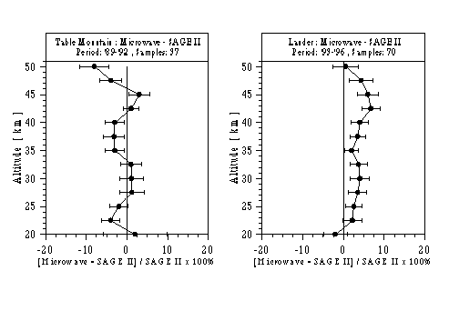
Figure 2.41 Mean of the relative differences between Microwave and SAGE II at Table Mountain from 1989 until 1992 (left panel) and at Lauder from 1993 until 1996 (right panel). Error bars are 2-sigma standard error.
The results of the comparison at Lauder are displayed in the right panel of Figure 2.41 and are based on 70 microwave/SAGE II coincidences. The mean difference is in the range +0-6% at altitudes between 20-50 km. Unlike the Table Mountain results, the sunrise and sunset comparisons are significantly different. The sunrise difference is about 5% larger at all altitudes than the sunset difference, suggesting that the sunrise measurements would be systematically smaller than the sunset measurements if they were sampling the same air. However, it is known that the microwave data at Lauder are affected by a bias of 1-3% during the observational period.
It is concluded that the ground-based microwave data shows good agreement with SAGE II and is a promising instrument for the future to validate and assess ozone trends in the stratosphere.
![]()