 |
Stratospheric Processes And their Role in Climate
|
||||||||
| Home | Initiatives | Organisation | Publications | Meetings | Acronyms and Abbreviations | Useful Links |
![]()
|
Stratospheric Processes And their Role in Climate
|
||||||||
| Home | Initiatives | Organisation | Publications | Meetings | Acronyms and Abbreviations | Useful Links |
![]()
Götz [1931] discovered that the ratio of zenith sky radiances of two wavelengths in the ultraviolet, one strongly and the other weakly absorbed by ozone, increases with increasing solar zenith angles but suddenly decreases at zenith angles close to 90o. He named this observation the Umkehr effect and realised that such measurements contain information about the vertical distribution of ozone in the stratosphere [Götz et al., 1934]. Umkehr observations today are performed with both Dobson [WMO, 1992; Staehelin et al., 1995] and Brewer [Kerr et al., 1988] spectrophotometers measuring the ratio of diffusely transmitted zenith-sky radiance at a wavelength pair in the ultraviolet, one wavelength strongly, the other weakly absorbed by ozone (e.g., for the C-wavelength pair, 311.5 nm is strongly absorbed and 332.4 nm weakly absorbed). These wavelength pairs are measured in a series of zenith-sky observations with the solar zenith angle changing from 60° to 90° during sunrise or sunset. During the Umkehr observation period, the Dobson or Brewer instrument also independently measures the total ozone column. The actual measurement vector consists of the logarithm of ratios of channel signals (R values) that are converted to radiance using calibrations tables [WMO, 1992; Kerr et al., 1996] and reported as N values in N-units for 12 discrete zenith angles between 60° and 90°. These measurements are inverted and archived as layer ozone amounts at the WOUDC.
The Dobson instrument employs a selection of eight wavebands from 305.5 to 339.8 nm [Komhyr et al., 1993] while the 8 Brewer wavebands occur between 306.3 and 329.5 nm [McElroy and Kerr, 1995]. Only the C-pair (311.5 and 332.4 nm) measurements are used in the current Dobson/Umkehr inversion [Mateer and DeLuisi, 1992], while the preliminary Brewer/Umkehr inversion uses either 5 or 6 wavebands [McElroy et al., 1996]. Both instrument retrievals use the Bass and Paur [1985] ozone absorption cross-sections.
The Umkehr inversions report ozone in 10 Umkehr layers (layers 0 and 1 are combined into layer 1) divided into equal log-pressure vertical intervals starting at the surface (1 atm.=1013 hPa) and extending to layer 10 (9.77x10⁻⁴ atm. to the top of the atmosphere). These Umkehr layers are approximately 5 km thick and are centred roughly at the layer number times 5 km in height (e.g. layer 8 is centred at 40 km). Although the standard Umkehr retrievals report 10 layers, because of a combination of the physical atmospheric scattering process, finite instrument spectral resolution, and real atmospheric vertical correlation, the actual retrievals possess, at most, 4 independent pieces of information (i.e., significant eigenvectors [Mateer, 1965, Hahn et al., 1995]). The vertical position and extent of this information is contained in the averaging kernels of the measurement technique, which are summarised in section 1.7.6. In general, the Umkehr technique retrieves ozone information between 20 and 40 km and is constrained to retrieve a profile consistent with the total ozone column measurement [Mateer and DeLuisi, 1992].
Of the approximately 90 Dobson stations world-wide, 46 Dobson stations have been used recently for total-ozone trend studies [Bojkov et al., 1995]. Because the Umkehr observations require much more observing time, only 19 stations are represented in the WOUDC database with Dobson/Umkehr observations. Of those, 15 stations (some of which are automated) have sufficiently long records to be initially considered in this study. These stations represent both hemispheres but are located predominantly in northern mid-latitudes. While some Dobson/Umkehr records extend back to 1957, the analyses in this report concentrate on the satellite-overlap period 1979-1996.
Because all of the instruments in the Brewer network, which now comprises more than 100 instruments, are automated, all Brewer stations report Umkehr measurements. Several Brewer stations have data records exceeding 10 years, sufficiently long to be used for trend studies [McElroy et al., 1996] and preliminary results compare favourably with other ozone instruments [McElroy and Kerr, 1995; Hahn et al., 1995]. However, the Brewer data require additional scientific effort to invert and validate before they can be used for trend studies. With appropriate inversion and validation, the Brewer records would have made a significant contribution to this report.
Sources of error in the Dobson instrument include optical alignment, optical wedge calibration, and detector noise. The Dobson instruments considered here are routinely calibrated for total ozone measurements with the world standard Dobson instrument 83, which maintains a long-term ( >25 year) precision of approximately ±0.5% [Komhyr et al., 1989; Basher, 1995]. This calibration of instrument 83 and the secondary standard instruments is maintained by both standard-lamp tests and Langley-plot calculations. While the Dobson instruments are routinely calibrated in the configuration for total ozone column measurements, they are not directly calibrated in the Umkehr mode. During measurements at high solar zenith angles, corresponding to ozone information at high altitudes, the instrument's internal scattered light level approaches the atmospheric signal. Therefore, instrument-to-instrument variability should be greatest in the upper-layer ozone retrievals. The resulting retrieval accuracy is discussed in section 1.7.6.
The current Umkehr inversion algorithm [Mateer and DeLuisi, 1992] is based on the techniques of Rodgers [1990] and represents the first update of the original (1964) algorithm [Mateer and Dütsch, 1964]. The measured N-values (defined below) are inverted to provide ozone amounts (in Dobson Units, DU) in 10 Umkehr layers through the application of a radiative transfer code that takes into account the primary and multiple atmospheric scattering, atmospheric refraction, and absorption by atmospheric ozone.
The Dobson zenith sky measurements may be written as
N(x,z) = 100 log10{[I(x,z,L2)/F0(L2)]/[I(x,z,L1)/F0(L1)]}+ C0
where N is the relative logarithmic attenuation for the wavelength pair and is referred to as the N-value. The quantity x refers to the ozone profile, z is the solar zenith angle, I(x,z,L1) is the 311.5 nm radiance and I(x,z,L2) is the 332.4 nm radiance of the C-wavelength pair, F0 is the extraterrestrial flux and C0 is an instrumental constant. In the forward model, the N-value comprises four components: the primary scattering component, Np, the multiple scattering component NMS, a refraction component NR, and an instrumental parameter C0.
Np = N – NMS – NR – Co
By using differences Yi = Ni - No, where Ni is the N-value at zenith angle zi and N0 the lowest zenith angle, C0 and the extraterrestrial flux can be eliminated.
The forward model uses the average of the M.A.P. 40°-50° North and South temperature profile with the temperature-dependent ozone cross sections of Bass and Paur [1985] and Paur and Bass [1985]. For the forward calculation, the atmosphere is divided into 61 layers in the vertical where each layer is 1/4 of the appropriate Umkehr layer. Table 1.11 shows the layer designations used in the Umkehr retrievals along with the pressure levels and approximate altitudes. The inverse model provides ozone content in 10 layers, where layer 10 includes all the ozone above layer 9, and layer 1 includes the retrieved ozone for both layers 0 and 1.
|
|
|
|
|
|
|
|
|
|
|
|
|
|
|
|
|
|
|
|
|
|
|
|
|
|
|
|
|
|
|
|
|
|
|
|
|
|
|
|
|
|
|
|
|
|
|
|
|
|
|
|
|
|
|
|
|
|
|
|
|
|
|
|
|
|
|
|
Table 1.11. Layers used for Umkehr ozone profile retrievals [Mateer and DeLuisi, 1992].
The inverse problem uses the observed N-value corrected for multiple scattering and refraction with the value for the smallest solar zenith angle subtracted. Additionally, the integral of the retrieved ozone is constrained to have the value of the observed total ozone. The retrieval algorithm uses the optimal estimation method of Strand and Westwater [1968] as formulated by Rodgers [1976]. At the nth iteration, retrieval xn+1 is obtained from xn by the following expression:
xn+1 = xA +[Sx-1+KnTSE-1Kn]-1KnTSE-1[(y–yn)–Kn(xA–xn)]
where xA is the a priori ozone profile, Sx is the covariance uncertainty matrix for the first guess profile, SE is the error covariance matrix for the measurements, yn is the vector of calculated observations for xn, Kn is the averaging kernel, and the superscript T represents matrix transposition.
The a priori profiles are significantly improved over the 1964 approximations. In layers above 5, these current a priori profiles are sinusoidal functions of Julian day and latitude in six latitude bands. The a priori amounts below layer 4 are quadratic functions of the measured total ozone amount only derived from ozonesonde climatology. The amounts in layers 4 and 5 result from a cubic fit to upper and lower layers.
The contributions to the error are from measurement errors, smoothing errors, forward-model errors, and inverse-model errors. The retrievals are also sensitive to the amount and distribution of atmospheric aerosols. Mateer and DeLuisi [1992] characterise the retrieval errors from various forward model inputs and from the inverse model. For a discussion of aerosol-induced errors see DeLuisi [1979] and Newchurch and Cunnold [1994]. The averaging kernels for an ozone column of 350 DU and a uniform Sx matrix appear in Figure 1.27. Although all Umkehr observations of all qualities are available in the WOUDC database, for comparative studies, one should restrict the population of retrievals to those with small differences between observed and fitted N values (rmsres 1.3 N units) and with convergence criteria dfrms 0.01 in the inversion process. These criteria affect profile comparisons more than trend studies.
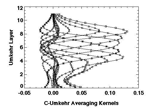
Figure 1.27. Averaging kernels from the 1992 C-Umkehr inversion algorithm for an ozone profile with 350 DU at 45oN using the uniform Sx covariance matrix. Ordinate labels represent the bottom of the designated layer. Symbols corresponding to retrieval layers are: layer 10, diamonds peaking at layer 8; layer 9, triangles peaking at layer 8; layer 8, squares peaking at layer 8; layer 7, crosses peaking at layer 7; layer 6, plusses peaking at layer 6; layer 5, asterisks peaking at layer 5; layer 4, diamonds peaking at layer 4; layer 3, triangles peaking at the top of layer 3; layer 2, squares peaking in layer 3, and layer 1, crosses peaking in layer 2.
Measurement errors
For a sufficiently large number of retrievals, one can calculate the error covariance matrix, SM given the measurement error covariance, SE, which adopts a variance of 1 (N-unit)2 for all zenith angles and 3 DU for the total ozone measurement. The result of this calculation indicates that above layer 9 there is no retrievable information. In the middle layers, measurement errors contribute 3-6% uncertainties to the profiles. In the lowest layers (3,2, and 1), retrieval errors increase.
Smoothing errors
Smoothing errors include profile structure that is either not seen or poorly seen in the Umkehr measurement. The smoothing error for layers 4 through 8 is approximately 10%. For layers below layer 4, it increases to 15% and for layers above 8 to 25%.
Forward model errors
Forward model errors include quadrature errors, parameter errors, and others such as the lack of inclusion of the effects of SO2 absorption, the failure to include multiple scattering in the partial derivative calculation, and the effect of temperature profile errors. Errors due to quadrature vary from 0.0 to 1.1% as a function of layer. The relevant parameters are the ozone absorption and Rayleigh scattering coefficients. Ozone errors due to reasonable uncertainties in these parameters range from 0.2% to 2.6% all functions of altitude. Errors due to heavy SO2 pollution (10 DU) result in ozone errors of approximately 3% in layers 4 through 8. Errors due to multiple scattering neglect in the partial derivative are generally less than 0.5% in layers 4-8 [Mateer and DeLuisi, 1992]; although in some cases the error maybe somewhat larger. Errors due to the assumption of a single temperature profile are less than ±3% and are strong functions of layer with a minimum less than 1% in layer 5 and increasing both above and below that layer.
Inverse model errors
Three areas that contribute to the inverse model errors are errors in the SE matrix, errors in the Sx matrix, and errors in the a priori profile. The first two jointly contribute about 1-4% uncertainty to the retrievals for levels between 4 and 8. The uncertainty is larger at levels above 8 and below 4.
Aerosol errors
The 1992 algorithm continues to be sensitive to atmospheric aerosols, particularly stratospheric aerosols. This aerosol interference is an optical effect caused by the scattering of light by the aerosols in the Junge aerosol layer (~20 km) on radiation that was initially scattered into the nadir by the atmosphere at much higher altitudes (e.g., 40 km for layer 8) [DeLuisi, 1979]. Ozone errors due to total aerosol optical depths of 0.016, with 0.012 of that atmospheric total in the stratosphere, are largest in layer 9. In layer 8, the error is approximately 4% with smaller errors in the other layers. For this reason, in this report we use only Umkehr with stratospheric aerosol optical depths less than 0.02 where the correction is less than approximately 6% and the uncertainty in that correction is on the order 1% in ozone amounts. This restriction results in omitting approximately one year of observations after both the eruptions of El Chichon and Mount Pinatubo but ensures minimal residual error due to aerosol interference.
A priori influence on trends
The determination of trends in layers below 5 is affected by a potential trend in the a priori profiles [Mateer et al., 1996]. Using differences in retrievals between synthetic and actual profiles the authors conclude that a time-dependent a priori profile would influence the calculated trend in layers 1-3 and somewhat in layer 4. Trends in layers above 4, however, are not affected by a potential trend in the a priori profile. The problem is moderated by using a time-dependent a priori ozone profile, combining layers 1, 2, and 3 into a single layer, and layers 8, 9, and 10 into a single layer. This finding is confirmed by the study of Petropavlovskikh et al. [1996a]. In this report, we take a somewhat more conservative approach and combine layers 1-4 into a single layer, but also calculate layers 4-8 separately. We then combine layers 8, 9, and 10 into a single 8+ layer. Alternative approaches could combine layers 1-3, 1-5, or 9-10.
The effect of appropriate errors on ozone trend calculations is summarised in Table 1.12. In layers 8 and 8+, the rss estimated error due to all sources on trend calculations is 0.23±0.21%/year diminishing to 0.2±0.2 %/year in layers 6, 5, and 4. The largest instrumental sources of uncertainty regarding trend estimation are the Umkehr calibration uncertainty and the aerosol optical interference correction.
|
|
%/ year |
%/year |
| Calibration | ||
| Total ozone |
|
|
| Umkehr |
|
|
| Smoothing Error | ||
| All sources |
|
|
| Forward Model | ||
| Quadrature |
|
|
| Spectroscopic parameters |
|
|
| SO2 absorption |
|
|
| Multiple scattering |
|
|
| Temperature (per K) |
|
|
| Inverse Model | ||
| SE matrix |
|
|
| Sx matrix |
|
|
| a priori profiles | ||
| layer4 |
|
|
| layers 5-8 |
|
|
| Aerosol Optical Interference | ||
| layers 8, 8+ |
|
|
| layers 7, 4- |
|
|
| layer 6 |
|
|
| layers 5, 4 |
|
|
| RSS Total | ||
| layers 8, 8+ |
|
|
| layers 7,4- |
|
|
| layers 6, 5, 4 |
|
|
Table 1.12. Error sources in trends calculated from Dobson/Umkehr ozone profile retrievals.
Correcting Umkehr observations for the high aerosol loads within 1 year after a major eruption requires sophisticated analysis. For example, DeLuisi et al. [1996] performed an extensive error analysis of the aerosol correction to the Umkehr ozone retrievals that included effects of size distribution errors, vertical profile errors, and errors using climatological profiles of ozone and aerosols. The result of this work clearly showed that the errors possess a non-linear dependence on the aerosol optical thickness. A linear multivariate regression analysis was conducted to examine the relationship between the aerosol load in one of the Umkehr layers to the retrieved ozone errors in all layers 1 through 10. The magnitude and sign of the contributions (absolute error) vary according to the amount of aerosol in the layer and the altitude location of the layer. The contribution of the aerosol in the layer with the maximum load (usually layer 4) produces a strong effect in all layers. For long-term trend studies, however, one can accurately correct the Umkehr observations in the linear part of the curve that occurs during smaller aerosol loadings and omit the enhanced aerosol periods (approximately 1 year after major eruptions).
Some questions remain concerning the accuracy of the Umkehr forward model, especially with regard to the treatment of multiple scattering. Petropavlovskikh et al. [1996b] compared various radiative transfer codes to evaluate the accuracy of the Dave scalar code used in the past to model the aerosol effect on the Umkehr retrieved ozone profile. The differences between the codes was found to be a function of the solar zenith angle of the calculation. They found that the calculated ozone errors are sensitive to the radiative transfer code adopted. The authors conclude that there are non-negligible differences between the results from the different codes and further study is warranted. Recent comparisons of Umkehr to SAGE profiles [Newchurch et al., 1997] indicates a discrepancy of approximately 5% between the Umkehr ozone columns and the SAGE columns (SAGE higher than Umkehr). This bias exhibits an altitude structure increasing from 0% in layer 4 to 15% in layer 8.
Under the auspices of the European Commission, the Umkehr data record from most stations world-wide is being reviewed to improve the retrieved profiles in several areas including the following: 1) instrumental calibration and compatibility with total ozone column measurements, 2) sensitivity to the temperature dependence of the ozone absorption cross sections, 3) a priori sensitivities, 4) aerosol corrections using satellite and ground-based aerosol measurements, and 5) comparisons to other ozone measurements. This work is an ambitious review and potential modification of essentially all important aspects of the Umkehr observations and ozone profile retrieval. It is currently in its early stages and has not affected the Umkehr database for the results reported here.
In summary, Dobson instruments produce long-term, well-calibrated measurements of ozone profiles in coarse vertical resolution in the stratosphere. The current retrieval uses the maximum likelihood formulation of Rodgers [1976], a priori ozone profiles as a function of latitude and Julian day, and the temperature-dependent ozone absorption coefficients of Bass and Paur, [1985]. It is a significant improvement over the previous inversion algorithm. The aerosol effect on the ozone retrievals can be accounted for at the expense of approximately one year of observations following major eruptions. The Brewer network comprises well-calibrated instruments some of which now have significant records that should be analysed for ozone trends after adequate scientific attention is given to the inversion algorithm and data validation.
![]()