• Introduction
• Model and experiments
• Results
• Relationships to the Arctic Oscillation
• Concluding remarks
• Acknowledgements
• References

FIGURES

• Figure 1
• Figure 2
• Figure 3
• Figure 4

Interannual variations of the general circulation and polar stratospheric ozone losses are investigated by using a general circulation model (GCM) developed at Kyushu University. The GCM includes simplified ozone photochemistry interactively coupled with radiation and dynamics in the GCM. Polar ozone depletion is brought about in the GCM by a parameterized ozone loss term. We performed an 'ozone depletion experiment' over successive 40 years with stratospheric ozone losses formed over the Arctic and Antarctic polar regions, along with a 'control experiment' which is a simulation without the ozone loss term. Results of the ozone depletion experiment show large interannual variations of the general circulation and polar ozone losses especially in the Northern Hemisphere winter and spring. It is found that the interannual variations are caused not only by dynamical conditions in the stratosphere, e.g., strength of the polar vortex and planetary wave activities, but also by interaction mechanisms between dynamical and ozone fields; the resultant interannual variability of the general circulation in the stratosphere becomes larger than that in the control experiment. Moreover, influences of the stratospheric ozone losses could extend to the troposphere; overall three-dimensional patterns of the interannual variations in dynamical fields seem to coincide well with those of the Arctic Oscillation.

Introduction

Recently, large ozone depletion has been observed during early spring over the Arctic. In particular, the ozone depletion during spring 1997 exhibits many similarities to the Antarctic ozone hole from the viewpoint of the ozone distribution as well as the stratospheric general circulation. Radiative and dynamical impacts of Antarctic ozone losses on the general circulation have been investigated by several authors [e.g., Mahlman et al., 1994]. Our recent study using an interactive ozone chemistry general circulation model (GCM) showed that Arctic ozone depletion also led to decreased solar ultraviolet (UV) heating and lower temperatures, resulting in a colder and stronger polar vortex, and brought about strengthening and continuation of ozone depletion itself [Hirooka et al., 1999a, b]. Interannual variability of ozone depletion was, however, much larger in the Arctic than in the Antarctic, because of larger variability of dynamical conditions, e.g., strength of the polar vortex and planetary wave activities. The main purpose of this study is to investigate relationship between interannual variation of ozone depletion and that of the general circulation, especially in the Northern Hemisphere winter-to-spring period.

Model and experiments

The GCM used in this study is a global spectral model developed at our laboratory, with triangle truncation at wavenumber 21 in the horizontal direction and 37 vertical layers extending from the surface to about 83 km. The GCM includes realistic topography and has a full set of physical processes, such as the boundary layer, hydrology, dry and moist convection, and radiative processes. Reyleigh friction and gravity wave drag parameterization are introduced for the zonal momentum equation to represent the drag force due to unresolved motions. The ozone mixing ratio is calculated for the region up to about 55 km on the basis of a parameterized Chapman cycle proposed by Hartmann [1978], in which the catalytic destruction of ozone due to HOx and NOx is parameterized through the tuning of reaction coefficients, whereas the ratio above that level is prescribed by climatological values. The ozone destruction near the surface is expressed by introducing a suitable deposition velocity around 1 km altitude. Hence, the ozone field is coupled interactively with the radiative and dynamical fields in the GCM. For details, see Miyahara et al. [1995].

In order to simulate the ozone depletion, a parameterized loss term is added in the continuity equation for the ozone mixing ratio. The loss term is switched on for the region between 120 and 16 hPa, when three conditions are met, i.e., a noontime zenith angle less than 85o, a temperature lower than 198 K, and a latitude higher than 54o. We performed here an 'ozone depletion experiment' including the loss term over successive 40 years, along with a 'control experiment' without the loss term over successive 20 years.

Results

Seasonal marches and their interannual variations

Figure 1 shows seasonal marches of zonal mean dynamical fields and ozone UV heating at several high latitudes in the Northern Hemisphere and levels. In each panel, green curve denotes the average for the ozone depletion experiment, while red curve denotes that for the control experiment. Vertical bars show standard deviations for each calendars day. It is found that zonal mean zonal winds and temperatures at 1 hPa for the both experiments show similar seasonal marches, whereas in the lower stratosphere they are largely different each other, especially for the temperature field. In the ozone depletion experiment, the temperature at 86o N and 54 hPa are kept cold well below the threshold value of the ozone loss term, 198 K, until the end of April, which is delayed by about 2 weeks comparing to the control experiment. This is connected with decreased ozone UV heating due to the Arctic ozone depletion. For a period from the beginning of the sunlit period (mid-March at 86o N) to the end of April, ozone UV heating in the ozone depletion experiment is smaller than that in the control experiment by a factor of 2. This is due mainly to the fact that the Arctic ozone losses occur almost every spring in the ozone depletion experiment.

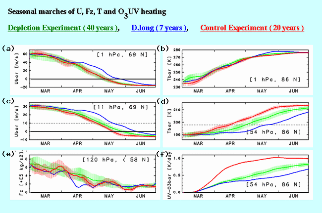
Figure 1. (a) Time series of the simulated zonal mean zonal wind at 69o N and 1 hPa. Green, blue and red lines denote averages for "ozone depletion experiment", "D.long years" (see the text) and "control experiment", respectively. Vertical bars for the green and red curves show standard deviations. (b) Same as (a) except for the zonal mean temperature at 86o N and 11 hPa. (c) Same as (a) except for the zonal mean zonal wind at 69o N and 11 hPa. Broken line indicates 10 ms-1. (d) Same as (a) except for the zonal mean temperature at 86o N and 54 hPa. Broken line indicates 198K. (e) Same as (a) except for the vertical component of E-P flux averaged over north of 58o N at 120 hPa. (f) Same as (a) except for the zonal mean ozone UV heating at 86o N and 54 hPa.

It is also noted that the interannual variation, expressed by the vertical bars, in the ozone depletion experiment is relatively large throughout the period, which is closely connected with the Arctic ozone depletion. Figure 2 shows the interannual variations of the date of polar vortex breakdown at 11 hPa, which is defined by the date when zonal mean zonal wind becomes smaller than 10 ms-1. Green circles show the breakdown date in the ozone depletion experiment, and red ones show those in the control experiment. The occurrence of final warmings in the ozone depletion experiment widely distributes for the period from mid-March to late June. As a result, in seven years denoted by blue circles, i.e. 2, 12, 15, 31, 35, 37, 40th years, the strong polar night jet and the Arctic ozone depletion continue harmonically until June. We call these seven years as 'D.long years' hereafter.

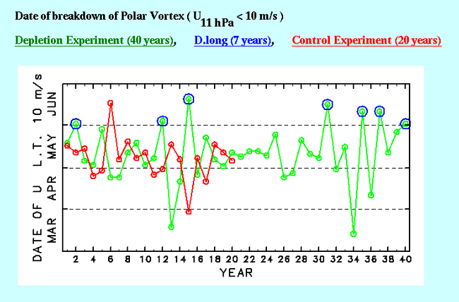
Figure 2. Interannual variation of date of breakdown of the polar vortex at 11 hPa. Green, blue and red circles denote the ozone depletion experiment, the D.long years (later than beginning of June) and the control experiment, respectively.

The blue curve in Fig. 1 shows the average of each field in the D.long years. Seasonal marches of the polar night jet, the polar temperature and the ozone UV heating in the lower stratosphere depart from each other from the latter half of April. In that period, the vertical component of Eliassen-Palm (E-P) flux in the lower stratosphere is smaller than other time series. Both the easterly acceleration due to E-P flux divergence in the upper stratosphere and the adiabatic heating related to descending motion are small in high latitudes in the stratosphere (not shown). After the period, final warmings occur in late May in the upper stratosphere, but relatively strong westerlies, low temperature and small ozone UV heating are maintained beyond the end of June in the lower stratosphere. Moreover, the strong polar night jet and the low temperature extend downward to the upper troposphere (not shown). It is also found that decrease of UV heating due to the ozone depletion in the polar lower stratosphere is a primary cause of the thermal structure, which leads to keeping the polar night jet strong until late spring. Similar to our former results [Hirooka et al., 1999a, b], this causes strengthening and continuation of the ozone depletion itself, through chemical destruction within the polar vortex and interfering dynamical transport of ozone-rich air from low latitudes. Hence, it is considered that the dynamically calm period in late April is a precursor for these positive feedback processes well shown in this experiment.

Relationships to the Arctic Oscillation

In order to investigate stratosphere-troposphere coupled interannual variation in the springtime seasonal march, a multiple empirical orthogonal function (M-EOF) analysis for the zonal mean zonal wind is conducted for each experiment. The EOF analysis is performed by combining multiple periods of data in a vector xi as

xi = ( ui(n), ui(n+1), ui(n+2), ui(n+3)),

where ui(n) is the anomalous period-mean zonal mean zonal wind at each height and latitude for the nth period of the ith year. The EOFs are then defined as the eigenvectors of the correlation matrix calculated from xi. The data in the north of 20o N and from 850 hPa to 0.1 hPa are used here. The EOFs are calculated for consecutive data of four period chosen as below; 1:APR 1-15, 2:APR 16-30, 3:MAY 1-15,4:MAY 16-30. It is noted that the calculation is conducted over 40 years data for the ozone depletion experiment, while done over 20 years data for the control experiment.

Figure 3 shows the first mode of the M-EOF (EOF1) obtained from above analysis, which accounts for 23.5% of variance. From green to blue colors show westerly anomalies, while yellow to red colors show easterly anomalies. Arrows show E-P flux vectors regressed with a time series of the EOF1, which are scaled for better visualization (the scaling factor is differed across 120 hPa). In the ozone depletion experiment (upper panels), a meridional dipole pattern of the zonal wind, which corresponds to the structure consisting of strong polar night jet in high latitudes and weak westerlies in subtropics, becomes strong and moves poleward and downward from the upper stratosphere to the troposphere with time, to form a barotropic structure similar to the so-called Arctic Oscillation [Thompson and Wallace, 1998]. On the other hand, in the troposphere, a reversed meridional dipole pattern comparing to the stratospheric one is found in the fist period; as the stratospheric dipole pattern moves downward, the polarity of the dipole in the troposphere is changed. In other words, a phase shift of the meridional structure occurs in relation to the stratospheric final warming.

Concerning E-P flux vectors corresponding to this mode, we can see that they direct toward two centers of easterly wind anomalies in the stratosphere and troposphere. In high latitudes, E-P flux vectors direct downward in April, while they reverse to the upward direction in May. This implies that in years when the polar night jet is kept strong until late spring, planetary wave activity in April is weak throughout the troposphere and the stratosphere, while in May it becomes strong. On the other hand, in the troposphere, poleward and downward vectors of the E-P flux converge in high latitudes to cause westerly acceleration in April, then meridional divergence and convergence formed by the poleward directed E-P flux moves easterly wind anomaly toward the subtropics until late May. As a result, the strong polar night jet extends from the lower stratosphere to the troposphere in late spring. Note that the zonal wavenumber 1 component is dominant in the vertical component of the E-P flux, whereas the zonal wavenumber 2 component is dominant for the meridional component in the troposphere, throughout the analysis period.

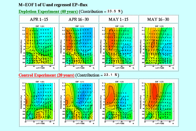
Figure 3. The M-EOF first mode for the zonal mean zonal wind, and regressed E-P flux. E-P flux vectors are scaled for better visualization by changing scaling factors across 120 hPa. Colors from green to blue represent westerly anomalies, from yellow to red show easterly anomalies. Horizontal axis shows latitude from 20o N to the north pole (from left to right). Vertical axis shows pressure from 850 hPa to 0.1 hPa.

On the other hand, EOF1 of the control experiment shows no systematic coupling of the stratosphere and the troposphere (lower panels in Fig.3). In this case the EOF1 accounts for 23.1% of variance. Although meridional dipole anomaly of the zonal wind moves poleward and downward in the stratosphere, it does not reach as deep as troposphere and becomes weak in late May. In the troposphere, meridional tripole pattern is seen throughout the period, and corresponding E-P flux vectors dominated by the zonal wavenumber 3 component cannot bring about a wind anomaly reverse. Hence in the ozone depletion experiment, the interannual variation of the polar night jet, which is enlarged by the positive feedback mechanism of the ozone depletion, extends to the troposphere to form the stratosphere-troposphere coupling, i.e. the Arctic Oscillation.

At the end of this section, it is interesting to see the time series of the EOF1 principal component. Figure 4 shows the time series of EOF1 along with dates of the breakdown of the polar vortex at 11 hPa, shown in Fig. 2. The time series of EOF1 is well correlated with dates of final warmings. It is found that extreme values which exceed a standard deviation of the principal component hardly appear in successive years, except for the 8th and 9th years in the ozone depletion experiment. In addition, these time series seem to have neither apparent periodicity nor trend, though no D.long years appeared for the 20-30th year period. Similar periods are considered to happen irregularly, because surface conditions of the GCM, such as SST, are fixed to climatology, and therefore there is no external memory or decadal forcing.

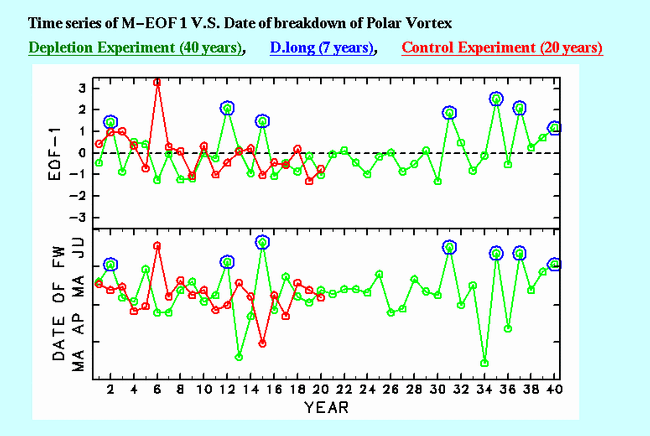
Figure 4. Upper: Time series of the standardized principal component of the EOF1. Green, blue and red circles denote those of the ozone depletion experiment, the D.long years (see the text) and the control experiment, respectively. Lower: Same as in Figure 2.

Concluding remarks

In the present study, it was shown that the resultant interannual variability of the general circulation in the stratosphere was larger than that in the control experiment, which is due mainly to the positive feedback mechanism of the Arctic ozone depletion. Moreover, influences of the stratospheric ozone losses extend to the general circulation in the troposphere. Concomitantly, the stratosphere-troposphere coupled interannual variation, which is extracted by the multiple EOF analysis for the springtime zonal mean zonal wind, shows a more systematic character than that in the control experiment.

Acknowledgments.

This work was supported by a Grant-in-Aid for the Cooperative Research with Center for Climate System Research, University of Tokyo, and by a Grant-in-Aid for Scientific Research from the Ministry of Education, Science, Culture and Sports, Japan. The GFD-DENNOU Library was used for drawing the figures.

References

Hartmann, D. L., A note concerning the effects of varying extinction on radiative-photochemical relaxation, J. Atmos. Sci., 35, 1125, 1978.

Hirooka, T., M. Yoshikawa, S. Miyahara, and T. Kayahara, Radiative and dynamical impacts of Arctic and Antarctic ozone holes: General circulation model experiments, Adv. Space Res., 24, 1637-1640, 1999a.

Hirooka, T., T. Nishiyoshi, S. Watanabe, and S. Miyahara, Influences of Arctic ozone hole on the stratospheric general circulation, Polar Meteorol. Glaciol., 13, 1-10, 1999b.

Mahlman, J. D., J. P. Pinto, and L. J. Umscheid, Transport, radiative and dynamical effects of the Antarctic ozone hole: A GFDL "SKYHI" model experiment, J. Atmos. Sci., 51, 489, 1994.

Miyahara, S., Y. Miyoshi, T. Kayahara, Y. Yoshida, M. Ooishi, and T. Hirooka, Development of a Middle Atmosphere General Circulation Model at Kyushu University, Climate System Dynamics and Modeling, Center for Climate System Research, University of Tokyo, pp. 75-103, 1995.

Thompson, D. W. J., and J. M. Wallace, The Arctic Oscillation signature in the wintertime geopotential height and temperature fields, Geophys. Res. Lett., 25, 1297-1300, 1998.