Department of Geophysics, Kyoto University, Kyoto, Japan
FIGURES
Abstract
1. Introduction
It has been observed that the global-scale stratospheric circulation has significant year-to-year variations in both hemispheres. The interannual variability is large during winter in Northern Hemisphere (NH), reflecting occurrence of stratospheric sudden warmings (SSWs) (e.g., Labitzke 1982). In Southern Hemisphere (SH), on the other hand, the variability is large in spring, depending on timing of the poleward and downward shift of the polar night jet (e.g., Shiotani et al. 1993).
Both observational and numerical studies have presented strong evidences that the variations in the stratosphere are coupled to those in the troposphere with each other in the contexts of SSWs and the Arctic Oscillation, that is, a deep signature of polar vortex modulation (see, e.g., Hartmann et al. 2000). These studies indicate that the troposphere and the stratosphere should be considered as a dynamically coupled system. However, fundamental nature of the troposphere-stratosphere (T-S) coupled system has not fully been understood.
In this study, therefore, we investigate internal intraseasonal and interannual variations of the T-S system in numerical experiments with a simple global circulation model under a periodic annual thermal forcing. No variations of external conditions, such as the 11-year solar cycle or interannual variations of the sea surface temperature, are included in the model. The results described below are based on two series of experiments (Taguchi and Yoden 2000a,b). One is a parameter sweep experiment, in which 100-year integrations are carried out by changing amplitude of a sinusoidal surface topography of zonal wavenumber one (100 years ¡ß10 runs). The other is a couple of millennium integrations, in which 1000-year integrations are done for each of two runs selected in the parameter sweep experiment (1000 years ¡ß2 runs).
2. Model
The model used in this study is a three dimensional global primitive-equation model with a resolution of T21L42. The seasonal cycle is included by Newtonian-type thermal relaxation toward a radiative equilibrium state which varies in time with an annual cycle. The model has other simplified physical processes; dry atmosphere with no moist processes, Rayleigh friction at the surface, and so on.
A sinusoidal surface topography of zonal wavenumber one is included. In the parameter sweep experiment, 100-year integrations are performed by changing the amplitude h0 of the topography from 0 m to 3000 m for 10 runs as an experimental parameter. In the millennium integrations, on the other hand, 1000-year integrations are done for two runs (h0 = 500 m and 1000 m) selected in the parameter sweep experiment, which have correspondence to the real atmosphere (SH and NH, respectively) in the stratospheric interannual variability.
3. Parameter Sweep Experiment
The parameter sweep experiment reveals that the stratospheric circulation depends on h0 in its mean seasonal march and interannual variability. The mean seasonal march of the zonal mean temperature in the polar upper stratosphere is highly dependent on h0 in cold seasons from autumn to spring (not shown). In the run of h0 = 0 m without the topography, the mean polar temperature only follows the annually-varying radiative forcing with a time lag of about several days. As h0 is increased to h0 ¡Á700 m, the polar temperature largely departs from the radiatively-determined state in spring, but the departure is small in winter. As h0 is further increased up to h0 = 3000 m, large departures appear in winter; the minimum temperature during the season becomes higher, while its timing becomes earlier.
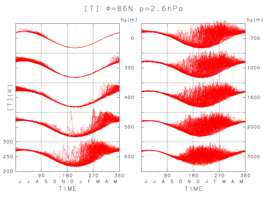
Interannual variability is large in different seasons dependent on h0 (Fig. 1). In the run of h0 = 0 m, the interannual variability is small in all seasons. As h0 is increased to h0 ¡Á500 m, the polar temperature comes to show large variability in spring. The variability is extremely large during winter in the runs of larger h0. These results remind us of the interannual variations in the real stratosphere; the interannual variability in the run of h0 = 500 m resembles that in the real SH stratosphere, while the variability in the run of h0 = 1000 m does that in the NH stratosphere.

Figure 1: Daily variations of the zonal mean temperature at ?Õ= 86N and p = 2.6 hPa for the 100 years in each run from h0 = 0 m to 3000 m.
4. Millennium Integrations
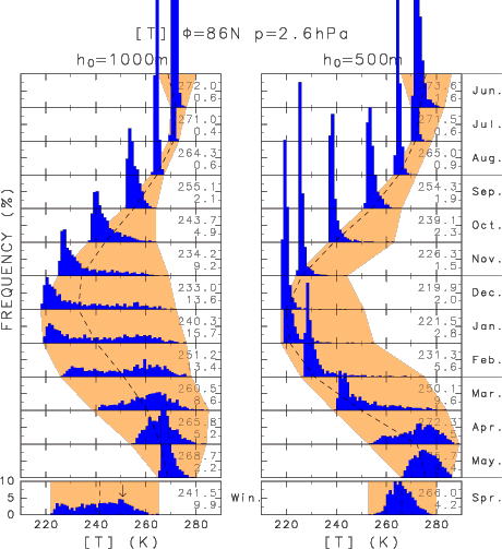
In the millennium integrations, statistically reliable frequency distributions of the monthly-mean polar temperature are obtained (Fig. 2). It is confirmed that interannual variability is very large during winter in the run of h0 = 1000 m (left), while it is large in spring in the run of h0 = 500 m (right). Also, the distributions are so smooth that they give information on their higher moments. The distributions in the run of h0 = 1000 m are positively skewed in autumn and bimodal in winter. On the other hand, those in the run of h0 = 500 have positive skewnesses for a longer period from autumn to spring; an extremely large skewness appears in March.

Figure 2: Frequency distributions of the monthly mean polar temperature in the two millennium integrations: h0 = 1000 m (left) and 500 m (right). Those for the winter mean for h0 = 1000 m and for the spring mean for h0 = 500 m are also displayed in the bottom. Averages and standard deviations for the 1000-year data are written on the right hand side of each panel (top and bottom numbers, respectively). The arrow in the winter mean (h0 = 1000 m) indicates a threshold value for the 200 years of highest temperature.
Intervals of warm winters, directly related to occurrence of SSWs,
are examined in the run of h0 = 1000 m by introducing a threshold value which determines the
top 200 highest winter-mean polar temperatures (indicated by the
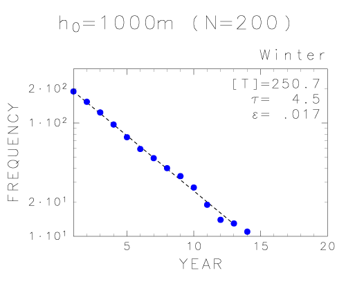
arrow in Fig. 2). Figure 3 displays frequency of intervals of
the warm winters, which persist for more than t years. The cumulated
frequency is surprisingly on a straight slope in the log-scale
plot, as well fitted by an exponential function A exp(-t/?Ó) (denoted
by the broken line). The broken line is determined by the least
square method, in which ?Óis estimated at 4.5 years. The good
fitting of the intervals by the exponential function means that
they are described by the exponential distribution. It, in turn,
indicates that the occurrence of warm winters itself is described
by the Poisson distribution. Both statistical distributions mean
that such warm winters occur at random from year to year. In these
distributions, ?Ó represents a mean interval, and hence, on average,
such warm winters take place once in 4.5 years. This nature of
random occurrence holds also for the spring-mean temperature (h0 = 500 m), independently of the choice of the threshold temperature.

Figure 3: Frequency distribution of intervals of warm winters, which persist for more than t years in the run of h0 = 1000 m. The warm winters are defined as the top 200 highest winter-mean polar temperatures (denoted by the arrow in Fig. 2). The border temperature is 250.7 K for the threshold. The broken line is the best-fit exponential function A exp(-t/?Ó), determined by the least square method. The mean interval ?Óis 4.5 years, and the mean error 0.017 (1 for one order).
Dominant modes of sequence of variability through one year are extracted with the empirical orthogonal function (EOF) analysis, which is applied to the polar temperature for the 12 months from June to May. In the run of h0 = 1000 m, the most dominant mode represents a variability of the minimum temperature in winter; the minimum temperature is higher than climatology (that is, occurrence of SSWs in winter) or lower (no SSWs). Intraseasonal variability in winter (second and third modes) and final warmings in March (fourth mode) are also important to the total variance. In the run of h0 = 500 m, on the other hand, most of interannual variability is related to the timing of the seasonal march from winter to spring; the seasonal march is earlier (warmings in March or April) or later (no warmings).
A lag-correlation (regression) analysis of SSWs shows a sequence of variability in the troposphere and the stratosphere, including preconditioning and aftereffect. One month before SSWs, the zonal mean zonal wind shifts poleward and planetary waves amplify in the troposphere and the stratosphere. The aftereffect is characterized by poleward and downward propagations of anomalies of the zonal mean zonal wind and planetary-wave amplitude, which continue for several months. This feature is basically the same as the slowly-propagating anomaly of the zonal mean zonal wind (e.g., Kodera 1995).
5. Concluding Remarks
Internal intraseasonal and interannual variations of the T-S coupled system has been investigated in numerical experiments with a simple global circulation model under a periodic annual forcing. Amplitude h0 of a sinusoidal surface topography of zonal wavenumber one is chosen as an experimental parameter.
The parameter sweep experiment of 100-year integrations for 10 runs (0 m ¡åh0 ¡å3000 m) shows that stratospheric interannual variability appears in different seasons dependent on h0. Some realistic variations are seen in two runs; the run of h0 = 500 m, in which the interannual variability is large in spring, corresponds to the real SH, while the run of h0 = 1000 m, in which the variability is very large in winter, do to the NH.
In the millennium integrations for the two runs, statistically reliable frequency distributions of the monthly mean temperature are obtained. By making use of the long datasets, it is found that warm winters due to SSWs occur at random from year to year. Dominant modes of interannual variability are extracted with the EOF analysis, and their differences between the two runs are emphasized. The T-S coupling is also examined with a lag-correlation analysis, which shows that the vertical coupling is inevitably two-way.
References
Hartmann, D. L., J. M. Wallace, V. Limpasuvan, D. W. J. Thompson, and J. R. Holton, 2000: Can ozone depletion and global warming interact to produce rapid climate change? Proc. Nat. Acad. Sci., 97, 1412-1417.
Kodera, K., 1995: On the origin and nature of the interannual variability of the winter stratospheric circulation in the northern hemisphere. J. Geophys. Res., 100, 14077-14087.
Labitzke, K., 1982: On the interannual variability of the middle stratosphere during the northern winters. J. Meteor. Soc. Japan, 60, 124-139.
Shiotani, M., N. Shimoda, and I. Hirota, 1993: Interannual variability of the stratospheric circulation in the southern hemisphere. Quart. J. Roy. Met. Soc., 119, 531-546.
Taguchi, M., and S. Yoden, 2000a: Internal intraseasonal and interannual variations of the troposphere-stratosphere coupled system in a simple global circulation model. Part I: Parameter sweep experiment. (in preparation)
Taguchi, M., and S. Yoden, 2000b: Internal intraseasonal and interannual variations of the troposphere-stratosphere coupled system in a simple global circulation model. Part II: Millennium integrations. (in preparation) .
Back to
| Session 1 : Stratospheric Processes and their Role in Climate | Session 2 : Stratospheric Indicators of Climate Change |
| Session 3 : Modelling and Diagnosis of Stratospheric Effects on Climate | Session 4 : UV Observations and Modelling |
| AuthorData | |
| Home Page | |