Previous: Parameter Sweep Experiment Next: Concluding Remarks Up: Ext. Abst.
4. Millennium Integrations
In the millennium integrations, statistically reliable frequency
distributions of the monthly-mean polar temperature are obtained
(Fig. 2). It is confirmed that interannual variability is very
large during winter in the run of h0 = 1000 m (left), while it is large in spring in the run of h0 = 500 m (right). Also, the distributions are so smooth that they
give information on their higher moments. The distributions in
the run of h0 = 1000 m are positively skewed in autumn and bimodal in winter.
On the other hand, those in the run of h0 = 500 have positive skewnesses for a longer period from autumn
to spring; an extremely large skewness appears in March.
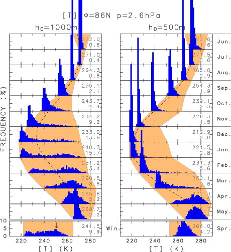
Figure 2: Frequency distributions of the monthly mean polar temperature
in the two millennium integrations: h0 = 1000 m (left) and 500 m (right). Those for the winter mean
for h0 = 1000 m and for the spring mean for h0 = 500 m are also displayed in the bottom. Averages and standard
deviations for the 1000-year data are written on the right hand
side of each panel (top and bottom numbers, respectively). The
arrow in the winter mean (h0 = 1000 m) indicates a threshold value for the 200 years of highest
temperature.
Intervals of warm winters, directly related to occurrence of SSWs,
are examined in the run of h0 = 1000 m by introducing a threshold value which determines the
top 200 highest winter-mean polar temperatures (indicated by the
arrow in Fig. 2). Figure 3 displays frequency of intervals of
the warm winters, which persist for more than t years. The cumulated
frequency is surprisingly on a straight slope in the log-scale
plot, as well fitted by an exponential function A exp(-t/?Ó) (denoted
by the broken line). The broken line is determined by the least
square method, in which ?Óis estimated at 4.5 years. The good
fitting of the intervals by the exponential function means that
they are described by the exponential distribution. It, in turn,
indicates that the occurrence of warm winters itself is described
by the Poisson distribution. Both statistical distributions mean
that such warm winters occur at random from year to year. In these
distributions, ?Ó represents a mean interval, and hence, on average,
such warm winters take place once in 4.5 years. This nature of
random occurrence holds also for the spring-mean temperature (h0 = 500 m), independently of the choice of the threshold temperature.
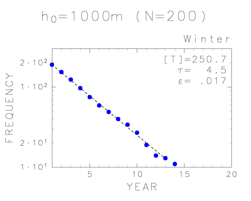
Figure 3: Frequency distribution of intervals of warm winters, which persist
for more than t years in the run of h0 = 1000 m. The warm winters are defined as the top 200 highest
winter-mean polar temperatures (denoted by the arrow in Fig. 2).
The border temperature is 250.7 K for the threshold. The broken
line is the best-fit exponential function A exp(-t/?Ó), determined
by the least square method. The mean interval ?Óis 4.5 years,
and the mean error 0.017 (1 for one order).
Dominant modes of sequence of variability through one year are
extracted with the empirical orthogonal function (EOF) analysis,
which is applied to the polar temperature for the 12 months from
June to May. In the run of h0 = 1000 m, the most dominant mode represents a variability of
the minimum temperature in winter; the minimum temperature is
higher than climatology (that is, occurrence of SSWs in winter)
or lower (no SSWs). Intraseasonal variability in winter (second
and third modes) and final warmings in March (fourth mode) are
also important to the total variance. In the run of h0 = 500 m, on the other hand, most of interannual variability is
related to the timing of the seasonal march from winter to spring;
the seasonal march is earlier (warmings in March or April) or
later (no warmings).
A lag-correlation (regression) analysis of SSWs shows a sequence
of variability in the troposphere and the stratosphere, including
preconditioning and aftereffect. One month before SSWs, the zonal
mean zonal wind shifts poleward and planetary waves amplify in
the troposphere and the stratosphere. The aftereffect is characterized
by poleward and downward propagations of anomalies of the zonal
mean zonal wind and planetary-wave amplitude, which continue for
several months. This feature is basically the same as the slowly-propagating
anomaly of the zonal mean zonal wind (e.g., Kodera 1995).
Previous: Parameter Sweep Experiment Next: Concluding Remarks Up: Ext. Abst.