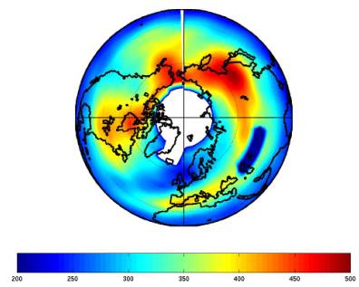
Figure 1: Total ozone on 15 February 1996 observed from GOME (left panel) and calculated by CTM2 (right). [Dobson Units]
(note: the dark blue area east of the Caspian Sea seen in the left panel is a region where no GOME data was available)
Department of Geophysics, University of Oslo, Norway
FIGURES
Abstract
1. Introduction
A new chemical transport model including both tropospheric and stratospheric chemistry has been developed for studies of chemical and dynamical processes in the tropopause region. Currently the model is used to calculate 3-D tracer distributions for 1996 and has been validated against observations from the same time. The field of possible applications is exemplified by two experiments that have been performed until now. In the first experiment the cross-tropopause flux of ozone was calculated and the effect of heterogeneous chemistry was assessed. The seasonal cycle of the tropospheric ozone budget was computed for cases including gas-phase chemistry only and including heterogeneous reactions on stratospheric sulphate aerosols and Polar Stratospheric Clouds (PSC). In the second experiment the effect of NOx emissions from civil subsonic aircraft on the distributions of ozone and reactive nitrogen was studied.
After a short description of the model and a validation against ozone measurements presented in sections 2 and 3, the two experiments will be described separately in sections 4.1 and 4.2. Section 5 will give a summary of the presented studies and outline plans for future development.
2. CTM2: Description of the model
The Oslo CTM2 isa global 3-dimensional chemical transport model (CTM) for the troposphere and the lower stratosphere, extending from the surface up to about 10 hPa where the uppermost layer is centered. The vertical grid comprises 19 layers defined in sigma-pressure hybrid coordinates, while the horizontal resolution can be varied between T21 (~5.6 °x5.6 °), T42 (~2.8 °x2.8 °), and T63 (~1.9 °x1.9 °).
However, all simulations for this paper have been performed with T21 resolution. The model meteorology is determined by a self-consistent set based on ECMWF forecast data including horizontal winds, temperature, cloud liquid water content, cumulus convection, etc. for the year 1996. Model results can thus be compared readily with observations from the same time (Sundet, 1997).
Advective transport uses the concept of Second Order Moments (Prather, 1986), while convection is based on the Tiedtke mass flux scheme (Tiedtke, 1987), where the vertical transport of species is determined by the surplus/deficit of mass flux in a column. Transport in the boundary layer is treated according to the Holtslag K-profile scheme (Holtslag et al., 1990).
Emissions of source gases (CO, NOx, Methane, VOC compounds) for different source categories are taken from the GEIA and EDGAR data bases for natural emissions, and from Mueller (1992) for anthropogenic emissions. High-altitude emissions of NOx from lightning and aircraft are included based on Price et al. (1997a/b) and the ÔIPCC-2001Õ aircraft inventory (IPCC, 2001), respectively. The calculation of dry deposition follows Wesely (1989). At the model top a constant mixing ratio boundary condition is applied using data from a multi-year simulation of the Oslo2D model.
For chemical integrations two separate modules are used covering tropospheric and stratospheric chemistry, respectively. The tropospheric chemistry scheme contains 51 species and has been thoroughly tested in the OSLO CTM-1 model (Berntsen and Isaksen, 1997). 86 thermal reactions, 17 photolytic reactions, and 2 heterogeneous reactions are integrated by the QSSA method (Hesstvedt et al., 1978) using a numerical time step of 5 minutes. The stratospheric chemistry solver is a well-tested extensive QSSA code developed by Stordal et al. (1985) and has been updated to include heterogeneous chemistry (Isaksen et al., 1990). It has been extensively used and validated in the OSLO 2D model (Isaksen et al., 1990) and in a stratospheric 3-D CTM (Rummukainen et al., 1999). 104 thermal, 47 photolytic, and 7 heterogeneous reactions involving a total of 57 species and 7 families are integrated in time steps of 10 minutes.
As a boundary between the tropospheric and the stratospheric chemistry regimes the 150ppbv ozone surface is chosen. Photodissociation rates are calculated on-line once every hour following the method described by Wild et al. (1999).
3. Model validation
Total ozone
GOME data has been collected from the ATMOS User Center at http://auc.dfd.dlr.de and compared with results obtained from CTM2 runs. Figure 1 shows a comparison for 15 February 1996.
Figure 1: Total ozone on 15 February 1996 observed from GOME (left panel) and calculated by CTM2 (right). [Dobson Units]
(note: the dark blue area east of the Caspian Sea seen in the left panel is a region where no GOME data was available)
When evaluating these results it has to be kept in mind that the uppermost layer of CTM2 contains only 2D data from the Oslo 2D model. Depending on latitude this layer is found to contribute between 15% (Poles) and 45% (low latitudes) to the total ozone column. Zonal variability of ozone occurring at altitudes above 20 hPa is not captured by CTM2, and yet, the agreement between CTM-2 and GOME is quite good, also in the Southern Hemisphere and during other seasons, for which no plots are shown here.
Vertical distribution of ozone
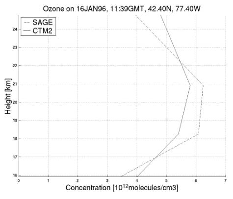
Height distributions of ozone were obtained by SAGE satellite observations and by LIDAR measurements at Andenes (Andøya, Northern Norway) for different heights and are compared with results from a CTM2 run. Figure 2 shows a comparison with SAGE data for 16 January 1996. The location of maxima agree well between model and observations. Also, the level agrees reasonably well with the exception of the 18 km altitude level where CTM2 overestimates the concentration of ozone by 50%.
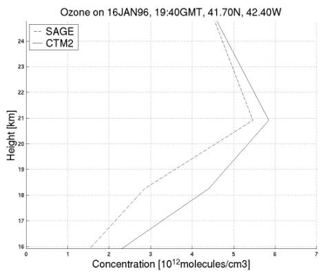
Figure 2: Comparison between SAGE satellite measurements of ozone with CTM2 data.
Figure 3 shows a time series plot for ozone at Andøya at two different altitudes. The level of ozone agrees well between observations and model. Deviations are assumed to be primarily due to the course horizontal resolution (T21). CTM2 nicely reproduces the high observed ozone levels at 25 km in the middle of March 1996 when Andøya was outside the Polar vortex, although the level is underestimated by about 15% in the beginning of this period.
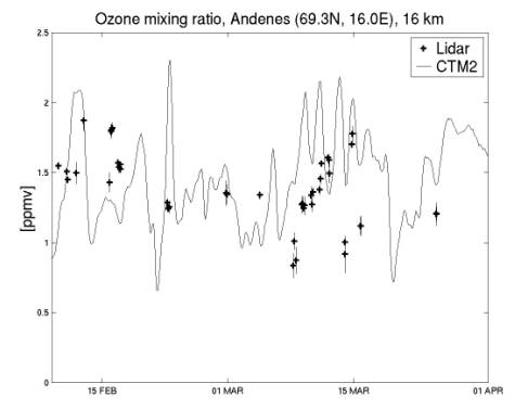
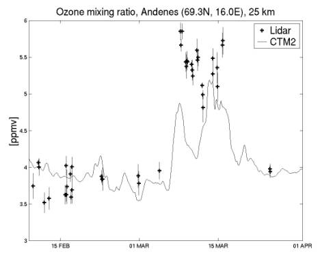
Figure 3: Comparison of ozone levels with LIDAR measurements at Andenes (Andøya, Northern Norway)
4. Experiments
4.1 Calculations of ozone flux through the tropopause
Including extensive chemistry modules for both the stratosphere and the troposphere and applying a highly accurate transport scheme CTM-2 is well-suited for calculations of cross tropopause fluxes of ozone, nitrogen oxides, and other chemical compounds. In addition, the effect of heterogeneous chemistry in the lower stratosphere on these fluxes and on photochemistry in the troposphere can be studied. Rate coefficients for heterogeneous reactions on sulphate aerosols are calculated by the scheme of Carslaw (1995). Gamma values for the reactions on PSCs are taken from JPL (2000). Sulphate aerosol data is retrieved from SAGE observations from 1989, which was a year with a relatively clean stratosphere (corresponding approximately to 1996). The modelled distribution of PSCs is confined to latitudes higher than 50 degrees and is based on temperature thresholds for PSC formation (<197 K at heights between 90 and 40 hPa, <193 K between 40 and 20 hPa) and the assumption of NAT particles with a mean radius of 1 micron and a mean density of 10 cm-3.
Figure 4 shows the tropospheric ozone budget for 1996 as obtained from a CTM-2 run including heterogeneous chemistry on stratospheric sulphate aerosols and PSCs. In addition (right panel) the tropopause flux is shown as a 30-day running mean, calculated in a run where heterogeneous chemistry in the stratosphere was switched off. All tropopause flux calculations use a climatological tropopause height based on NCEP data and made available at the SPARC Data Center (http://www.sparc.sunysb.edu).
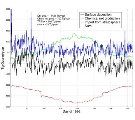
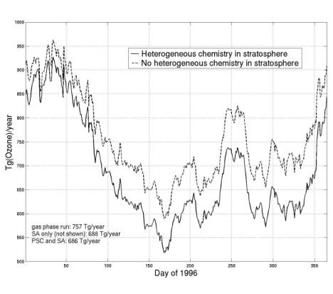
Figure 4: Left panel: Tropospheric ozone budget showing diurnal means of dry deposition, import from the stratosphere, chemical net production and the sum scaled to Tg(ozone)/year. Right panel: Cross tropopause flux plotted as 30-day running mean for the run including heterogeneous chemistry and a simulation with gas-phase reactions only.
As can be seen the cross tropopause flux is increased in the absence of heterogeneous reactions due to higher ozone levels of ozone.
PSCs which cover only a small fraction of the EarthÕs surface during short time periods have only little effect on the tropopause flux in this simulation: 686 Tg(Ozone)/year are calculated if both PSC and SA reactions are included, while 688 Tg(Ozone)/year is the result when PSC reactions are switched off. The effect of PSCs on the globally integrated tropopause flux is most pronounced during spring in the Southern Hemisphere. Stratospheric aerosol has global coverage and is present in all seasons. Globally integrated tropopause flux is therefore sensitive to the inclusion of heterogeneous chemistry on these particles. The right panel of Figure 4 also illustrates the dominance of the Northern Hemisphere regarding downward transport of ozone during the winter season.
4.2 Effect of aircraft emissions
As mentioned above, CTM2 includes NOx emissions from aircraft based on the ÔIPCC 2001Õ (IPCC, 2001) scenario. These emissions were retrieved from the 1992 data provided by NASA and scaled up to 2000 conditions. In order to study the effect of NOx from aircraft a run without emissions from aircraft emissions was performed. Figure5 shows the increase in NOy and ozone due to aircraft emissions of NOx. Figure 6 shows the ozone net production in the UTLS region and changes resulting from aircraft emissions. NOx emissions from aircraft result in higher ozone production except for the regions where NOx levels and ozone production are modeled to have high background values (South-Eastern China).
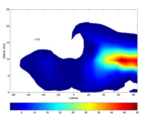
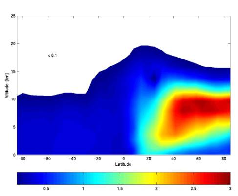
Figure 5: Left panel: Change in zonal-mean NOy due to aircraft emissions, June 1996 [%]. Right panel: Change in zonal-mean ozone due to aircraft emissions, June 1996 [%].
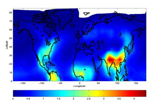
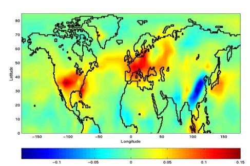
Figure 6: Left panel: Chemical net production of ozone integrated from 450 hPa to 120 hPa. Right panel: Change in chemical net production of ozone due to aircraft integrated over the same height region. The unit in both panels is 1011 molecules/(s*cm2).
Also, the flux of reactive nitrogen (NOy=NO+NO2+NO3+N2O5+HNO4+ClONO2+BrONO2+HNO3) through the tropopause has been calculated for both runs (see Figure 7).
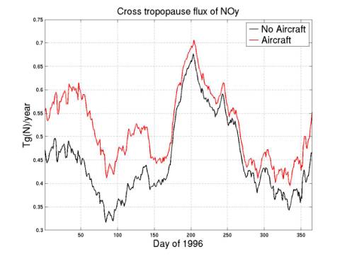
Figure 7: Cross tropopause flux of NOy.
Aircraft emissions increase the cross tropopause flux of NOy. This effect is most pronounced (up to 20%) between January and May when the tropopause height is relatively low at Northern mid latitudes and, as a consequence, a greater fraction of aircraft emissions occurs in the lower stratosphere rather than in the upper troposphere.
5. Summary and future plans
Globally integrated flux of ozone has been shown to depend on heterogeneous chemistry on stratospheric aerosol. The model calculates 686 Tg(Ozone)/year when heterogeneous chemistry on stratospheric aerosol and PSCs is included. Without heterogeneous chemistry in the stratosphere this value increases to 757 Tg(Ozone)/year.
Ozone and NOy are significantly increased in the UTLS region due to air traffic. The downward flux of NOy through the tropopause is very sensitive to emissions of aircraft occurring in the stratosphere.
Preparations are now going on for use of meteorological data from a 40-layer forecast model extending from the surface, by which the vertical resolution in the lower stratosphere will be improved by a factor of two. Furthermore, upper boundary conditions are going to be based on observations rather than data from the Oslo 2D model. Alternatively the model domain could be extended up to 0.1 hPa by use of the ECMWF 60 layer model.
Regarding chemistry the following possibilities we consider the inclusion of:
· a microphysical scheme for a more detailed description of particle formation and distribution
· particle sedimentation from the lower stratosphere into the troposphere (dehydrification/denitrification)
6. Acknowledgements
This study has been made possible by a funding of the Norwegian Research Council in the framework of the COZUV project (Coordinated project on Ozone and UV). The authors would also like to thank the ATMOS User Center and the SPARC Data Center for making available observational and climatological data used in this study, and Georg Hansen (NILU, Norway) for providing data from LIDAR measurements made at Andøya.
7. References
Berntsen T. and I. S. A. Isaksen, A global 3-D chemical transport model for the troposphere, 1, Model description and CO and Ozone results, J. Geophys. Res., 102, 21.239-21.280, 1997.
Hesstvedt E., O. Hov, I.S.A Isaksen, Quasi steady-state approximation in air pollution modelling: Comparison of two numerical schemes for oxidant prediction, Int. Journal of Chem. Kinetics, Vol. X, 971 994, 1978.
Holtslag, A. A. M., E. I .F DrBruijn and H.-L. Pan, A High resolution air mass transformation model for short-range weather forecasting, Mon. Wea. Rev., 118, 1561-1575, 1990.
Intergovernmental Panel on Climate Change (IPCC),WGI Third Assessment Report, in preparation, 2001.
Isaksen, I.S.A., Rognerud, B., Stordal, F., Coffey, M.T. and Mankin, W.G., Studies of Arctic stratospheric ozone in a 2-d model including some effects of zonal asymmetries. Geophys. Res. Lett., 17, p. 557-560, 1990.
Mclinden C. A, S. Olsen, B. Hannegan, O. Wild, M. J. Prather and J. Sundet, Stratospheric Ozone in 3-d Models: A simple chemistry and the cross-tropopause flux, J. Geophys. Res., Accepted January, 2000.
Moeller, J., Geographical distribution and seasonal variation of surface emissions and deposition velocities of atmospheric trace gases. J. Geophys. Res., 97, 3787-3804, 1992.
Prather, M. J., Numerical advection by conservation of second-order moments, J. Geophys. Res., 91, 6671-6681, 1986.
Price C., J. Penner and M. Prather, NOx from lightning 1. Global distribution based on lightning physics. J. Geophys. Res., 102, p. 5929-5241, 1997a.
Price C., J. Penner and M. Prather, NOx from lightning 2. Constraints from the global atmospheric circuit. J. Geophys. Res., 102, p. 5943-5251, 1997b.
Rummukainen, M., Isaksen, I.S.A., Rognerud, B., and Stordal, F., A global model tool for three-dimensional multiyear stratospheric chemistry simulations: Model description and first results. J. Geophys. Res., 104, p.26437-26456, 1999.
Stordal, F., Isaksen, I.S.A. and Horntvedt, K., A diabatic circulation two-dimensional model with photochemistry: Simulations of ozone and long-lived tracers with surface sources. J. Geophys. Res., 90, p. 5757-5776, 1985.
Sundet, J. K., Model Studies with a 3-d Global CTM using ECMWF data.Ph.D. thesis, Dept. of Geophysics, University of Oslo, Norway, 1997.
Tiedtke, M., A Comprehensive Mass Flux Scheme for Cumulus Parameterisation on Large Scale Models, Mon. Wea., Rev., 117, 1779-1800, 1989.
Wesley, M. L.,Parameterization of surface resistances to gaseous dry deposition in regional-scale numerical models. Atmos. Environ., 23, 1293-1304, 1989.
Wild O., X. Zhu and M. J. Prather: Fast-J: Accurate simulation of in- and below cloud photolysis
in global chemical models, J. Atmos. Chem, Submitted December, 1999.
Back to
| Session 1 : Stratospheric Processes and their Role in Climate | Session 2 : Stratospheric Indicators of Climate Change |
| Session 3 : Modelling and Diagnosis of Stratospheric Effects on Climate | Session 4 : UV Observations and Modelling |
| AuthorData | |
| Home Page | |