S P A R C Stratospheric Processes And their Role in Climate A project of the World Climate Research Programme Home Initiatives Organisation Publications Meetings Acronyms and Abbreviations Useful Links

Assimilation of Stratospheric Meteorological and
Constituent Observations: A Review

Richard B. Rood, NASA Goddard Space Flight Center, USA (Richard.B.Rood@nasa.gov)

Introduction

The assimilation of stratospheric observations has been the focus of several research groups in the past fifteen years. The use of products from the assimilation of meteorological data is now widespread. As new data types become available researchers are anxious to try assimilation experiments. This article will review progress in the last 3-5 years and evaluate that progress in terms of the underlying geophysical robustness of data assimilation systems.

A dictionary definition of assimilation is: to incorporate or absorb, for instance, into the mind or the prevailing culture. For Earth science, assimilation is the incorporation of observational information into a physical model. Or more specifically, data assimilation is the objective melding of observed information with model-predict-ed information.

Assimilation rigorously combines statistical modelling with physical modelling. Daley (1991) is the standard text on data assimilation. Cohn (1997) explores the theory of data assimilation, and its foundation in estimation theory. Swinbank et al. (2003) is a collection of tutorial lectures on data assimilation. Assimilation is difficult to do well, easy to do poorly, and its role in Earth science is expanding and sometimes controversial.

In the atmosphere the predominant observations that are assimilated are temperatures, or radiances that represent the temperature. These observations come from radiosondes, aircraft and satellites. Wind data are also assimilated, and are of crucial importance to the quality of the assimilation. As a function of altitude the amount of wind data available for assimilation drops dramatically above the tropopause. Hence, the state of the stratosphere is determined primarily by temperature observations and information propagated from the surface and the troposphere. A good tropospheric assimilation is required for a good stratospheric assimilation.

A number of constituents are also of interest. Water vapour has been routinely assimilated in the troposphere for many years and is important to the specification of tropospheric physics. More recently, several centres and groups have undertaken the assimilation of ozone. There have also been a number of experiments addressing interacting chemical species. Both ozone assimilation and chemical assimilation are reviewed in Swinbank et al. (2003).

There are a number of factors that motivate the desire to assimilate geophysical parameters. The list below is specifically for ozone, but it is representative of the motivation of other geophysical parameters as well.

Motivations for Ozone Assimilation

- Mapping: There are spatial and temporal gaps in the ozone observing system. A basic goal of ozone assimilation is to provide vertically resolved global maps of ozone.

- Short-term ozone forecasting: There is interest in providing operational ozone forecasts in order to predict the fluctuations of ultraviolet radiation at the surface of the earth (Long et al., 1996).

- Chemical constraints: Ozone is important in many chemical cycles. Assimilation of ozone into a chemistry model provides constraints on other observed constituents and helps to provide estimates of unobserved constituents.

- Unified ozone data sets: There are several sources of ozone data with significant differences in spatial and temporal characteristics as well as their expected error characteristics. Data assimilation provides a potential strategy for combining these data sets into a unified data set.

- Tropospheric ozone: Most of the ozone is in the stratosphere, and tropospheric ozone is sensitive to surface emission of pollutants. Therefore, the challenges of obtaining accurate tropospheric ozone measurements from space are significant. The combination of observations with the meteorological information provided by the model offers one of the better approaches available to obtain global estimates of tropospheric ozone.

- Improvement of wind analysis:The photochemical time scale for ozone is long compared with transport timescales in the lower stratosphere and upper troposphere. Therefore ozone measurements contain information about the wind field that might be obtained in multi-variate assimilation.

- Radiative transfer: Ozone is important in both longwave and shortwave radiative transfer. Therefore accurate representation of ozone is important in the radiative transfer calculations needed to extract (retrieve) information from many satellite instruments. In addition, accurate representation of ozone has the potential to impact the quality of the temperature analysis in multi-variate assimilation.

- Observing system monitoring:Ozone assimilation offers an effective way to characterize instrument performance relative to other sources of ozone observations as well as the stability of measurements over the lifetime of an instrument.

- Retrieval of ozone: Ozone assimilation offers the possibility of providing more accurate initial guesses for ozone retrieval algorithms than are currently available.

- Assimilation research: Ozone (constituent) assimilation can be productively approached as a univariate linear problem. Therefore it is a good framework for investigating assimilation science; for example, the impact of flow dependent covariance funcions.

- Model and observation validation: Ozone assimilation provides several approaches to contribute to the validation of models and observations.

Some of the goals mentioned above can be meaningfully addressed with the current state of the art, others cannot. It is straightforward to produce global maps of total column ozone which can be used in, for instance, radiative transfer calculations. The use of ozone measurements to provide constraints on other reactive speciesis an application that has been explored since the 1980’s (see Jackman et al., 1987) and modern data assimilation techniques potentially advance this field. The impact of ozone assimilation on the meteorological analysis of temperature and wind, and hence improvement of the weather forecast, is also possible. The most straightforward impact would be on the temperature analysis in the stratosphere. The improvement of the wind analysis is a more difficult challenge and confounded by the fact that where improvements in the wind analyses are most needed, the tropics, the ozone gradients are relatively weak. The use of ozone assimilation to monitor instrument performance and to characterize new observing systems is currently possible and productive (see Stajner et al., 2004). The improvement of retrievals using assimilation techniques to provide ozone first guess fields that are representative of the specific environmental conditions is also an active research topic. The goal of producing unified ozone data sets from several instruments is of little value until bias can be correctly accommodated in data assimilation. This final topic will be discussed more fully below.

In order to discuss why assimilation is successful in addressing some of these goals and less successful in others, the underlying physical foundation of assimilation will be considered. This will be based on the discussion of modelling and assimilation and comparison of the attributes of the concepts of performing simulation (modelling) and assimilation. Following this, expository examples will be presented. An underlying tenet is that by comparing results from a simulation to results from an assimilation using the same model, the researcher is investigating cause and effect in a controlled experiment.

TOP

Simulation and Assimilation

In order to provide an overarching background for thinking about model simulation, it is useful to consider the elements of the modelling, or simulation, framework described in Table 1. In this framework are six major ingredients. The first is the specification of boundary and initial conditions (e.g. topography and sea surface temperatures for an atmospheric model). Boundary conditions are generally prescribed from external sources of information.

The next three items in the table are intimately related. They are the representative equations, the discrete or parameterized equations, and the constraints drawn from theory. The representative equations are the analytic form of forces or factors that are considered important in the representation of the evolution of a set of parameters. All of the analytic expressions used in atmospheric modelling are approximations; therefore, even the equations the modeller is trying to solve have a priori errors. That is, the equations are scaled from some more complete representation, and only terms that are expected to be important are included in the analytic expressions (see Holton, 2004). The solution is, therefore, a balance amongst competing forces and tendencies. Most commonly, the analytic equations are a set of nonlinear partial differential equations.

The discrete or parameterized equations arise because it is generally not possible to solve the analytic equations in closed form. The strategy used by scientists is to develop a discrete representation of the equations which are then solved using numerical techniques. These solutions are, at best, discrete estimates to solutions of the analytic equations. The discretization and parameterization of the analytic equations introduce a large source of error. This introduces another level of balancing in the model; namely, these errors are generally managed through a subjective balancing process that keeps the numerical solution from running away to obviously incorrect estimates.

While all of the terms in the analytic equation are potentially important, there are conditions or times when there is a dominant balance between, for instance, two terms. An example of this is thermal wind balance in the middle latitudes of the stratosphere (see Holton, 2004). It is these balances, generally at the extremes of spatial and temporal scales, which provide the constraints drawn from theory. If the modeller implements discrete methods which consistently represent the relationship between the analytic equations and the constraints drawn from theory, then the modeller maintains a substantive scientific basis for the interpretation of model results.

The last two items in Table 1 represetn the products that are drawn from the model.  These are divided into two types: primary products and derived products. The primary products are variables such as wind, temperature, water, ozone – parameters that are most often, explicitly modelled; that is, an equation is written for them. The derived products are often functional relationships between the primary products; for instance, potential vorticity (Holton, 2004). A common derived product is the balance, or the budget, of the different terms of the discretized equations. The budget is then studied, explicitly, on how the balance is maintained and how this compares with budgets derived directly from observations. In general, the primary products can be directly evaluated with observations and errors of bias and variability estimated. If attention has been paid in the discretization of the analytic equations to honour the theoretical constraints, then the derived products will behave consistently with the primary products and theory. They will have errors of bias and variability, but they will behave in a way that supports scientific scrutiny.

In order to explore the elements of the modelling framework described above, the following continuity equation for a constituent, A, will be posed as the representative equation. The continuity equation represents the conservation of mass for a constituent and is an archetypical equation of geophysical models. Brasseur and Solomon (1986) and Dessler (2000) provide good backgrounds for understanding atmospheric chemistry and transport. The continuity equation for A is:

∂A/∂t = –Ñ·UA + M + P – LA – n/HA + q/H (1)

where A is some constituent, U is velocity (“resolved” transport, “advection”), M is “Mixing” (“unresolved” transport, parameterization), P is production, L is loss, n is “deposition velocity”, q is emission, H is representative length scale for n and q, t is time, and ?is the gradient operator.

Attention will be focused on the discretization of the resolved advective transport. Figures 1 and 2 illustrate the basic concepts. On the left of the figure a mesh has been laid down to cover the spatial domain of interest. In this case it is a rectangular mesh. The mesh does not have to be rectangular, uniform, or orthogonal. In fact the mesh can be unstructured or can be built to adapt to the features that are being modelled. The choice of the mesh is determined by the modeller and depends upon the diagnostic and prognostic applications of the model (see Randall, 2000). The choice of mesh can also be determined by the computational advantages that might be realized.

Points can be prescribed to determine location with the mesh. In Figure 1 both the advective velocity and the constituent are prescribed at the centre of the cell. In Figure 2, the velocities are prescribed at the centre of the cell edges, and the constituent is prescribed in the centre of the cell. There are no hard and fast rules about where the parameters are prescribed, but small differences in their prescription can have a huge impact on the quality of the estimated solution to the equation, i.e. the simulation. The prescription directly impacts the ability of the model to represent conservation properties and to provide the link between the analytic equations and the theoretical constraints (see Rood, 1987; Lin and Rood, 1996; Lin, 2004). In addition, the prescription is strongly related to the stability of the numerical method; that is, the ability to represent any credible estimate at all.

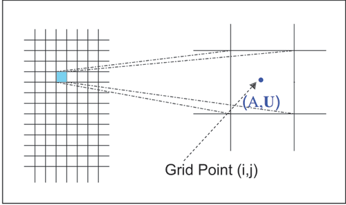Figure 1:Discretization of resolved transport and the choice of where to represent information impacts the physics, such as conservation,  scale analysis limits, and stability (Rood, 1987).  Grids may be orthogonal, uniform area, adaptive, or unstructured. For better resolution, please contact the SPARC Office.

Figure 1:Discretization of resolved transport and the choice of where to represent information impacts the physics, such as conservation,  scale analysis limits, and stability (Rood, 1987).  Grids may be orthogonal, uniform area, adaptive, or unstructured. For better resolution, please contact the SPARC Office.

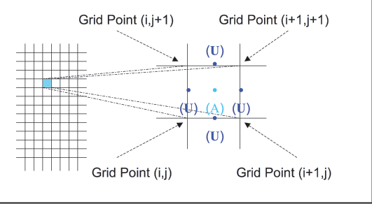Figure 2: Another choice of where to represent information on the grid. For better resolution, please contact the SPARC Office.

The use of numerical techniques to represent the partial differential equations that represent the model physics is a straightforward way to develop a model. There are many approaches to discretization of the dynamical equations that govern geophysical processes (Jacobson, 1998; Randall, 2000). One approach that has been recently adopted by several modelling centres is described in Lin (2004). In this approach the cells are treated as finite volumes and piecewise continuous functions are fit locally to the cells. These piecewise continuous functions are then integrated around the volume to yield the forces acting on the volume. This method, which was derived with physical consistency as a requirement for the scheme, has proven to have numerous scientific advantages. The scheme uses the philosophy that if the physics are properly represent then the accuracy of the scheme can be robustly built on a physical foundation.

Table 2 shows elements of an assimilation framework that parallels the modelling elements in Table 1. The concept of boundary conditions remains the same; that is, some specified information at the spatial and temporal domain edges. Of particular note, the motivation for doing data assimilation is often to provide the initial conditions for predictive forecasts.

Data assimilation adds an additional forcing to the representative equations of the physical model; namely, information from the observations. This forcing is formally added through a correction to the model that is calculated, for example, by (see Stajner et al., 2001):

(OPfOT + R)x = Ao – OAf(2)

The terms in the equation are as follows: Aoare observations of the constituent, Aƒ are model forecast (simulated estimates of the constituent, often called the first guess), Ois the observation operator, Pƒ is the error covariance function of the forecast, R is the error covariance function of the observations, x is the innovation that represents the observation-based correction to the model, and ( )T is the matrix transform operation. The observation operator, O, is a function that maps the parameter to be assimilated into observation space.

The error covariance functions Pƒ and R represent the errors of the information from the forecast model and the information from the observations, respectively. This explicitly shows that data assimilation is the error-weighted combination of information from two primary sources. From first principles, the error covariance functions are prohibitive to calculate. Stajner et al. (2001) show a method for estimating the error covariances in an ozone assimilation system.

Parallel to the elements in the simulation framework (Table 1), discrete numerical methods are needed to estimate the errors as well as to solve the matrix equations in Equation (2). Addressing physical constraints from theory is a matter of both importance and difficulty. Often, for example, it is assumed that the increments of different parameters that are used to correct the model are in some sort of physical balance. For instance, wind and temperature increments might be expected to be in geostrophic balance. However, in general, the data insertion process acts like an additional forcing term in the equation, and contributes a significant portion of the budget. This explicitly alters the physical balance defined by the representative equations of the model. Therefore, there is no reason to expect that the correct geophysical balances are represented in an assimilated data product. This is contrary to the prevailing notion that the model and observations are ‘consistent’ with one another after assimilation.

The final two elements in Table 2 are, again, the products. In a good assimilation the primary products, most often the prognostic variables, are well estimated. That is, both the bias errors and the variance errors are reduced relative to the model simulation. However, the derived products are likely to be physically inconsistent because of the nature of the corrective forcing added by the observations. These errors are often found to be larger than those in self-determining model simulations. This is of great consequence as many users look to data assimilation to provide estimates of unobserved or derived quantities. Molod et al. (1996) and Kistler et al. (2001) provide discussions on the characteristics of the errors associated with primary and derived products in data assimilation systems.

As suggested earlier, the specification of forecast and model error covariances and their evolution with time is a difficult problem. In order to get a handle on these problems it is generally assumed that the observational errors and model errors are unbiased over some suitable period of time, e.g. the length of the forecast between times of data insertion. It is also assumed that the errors are in a Gaussian distribution. The majority of assimilation theory is developed based on these assumptions, which are, in fact, not valid assumptions. In particular, when the observations are biased, there would be the expectation that the actual balance of geophysical terms is different from the balance determined by the assimilation. Furthermore, since the biases will have spatial and temporal variability, the balances determined by the assimilation are quite complex. Aside from biases between the observations and the model prediction, there are biases between different observation systems for the same parameters. These biases are potentially correctible if there is a known standard of accuracy defined by a particular observing system. However, the problem of bias is a difficult one to address and perhaps the greatest challenge facing assimilation (see, Dee and da Silva, 1998).

As a final general consideration, there are many time scales represented by the representative equations of the model. Some of these time scales represent balances that are achieved almost instantly between different variables. Other time scales are long (e.g. the general circulation), which will determine the distribution of long-lived trace constituents. It is possible in assimilation to produce a very accurate representation of the observed state variables, and those variables which are balanced on fast time scales. On the other hand, improved estimates in the state variables are found, at least sometimes, to be associated with degraded estimates of those features determined by long time scales. Conceptually, this can be thought of as the impact of bias propagating through the physical model. With the assumption that the observations are fundamentally accurate, this indicates errors in the specification of the physics that demand further research.

TOP

Transport applications: What have we learned?

Rood et al. (1989) first used winds and temperatures from a meteorological assimilation to study stratospheric transport. Since that time there have been productive studies of both tropospheric and stratospheric transport. However, a number of barriers have been met in recent years, and the question arises - has a wall been reached where foundational elements of data assimilation are limiting the ability to do quantitative transport applications? Stohl et al. (2004; and references therein) provide an overview of some of the limits that need to be considered in transport applications.

In transport applications, winds and temperatures are taken from a meteorological assimilation and used as input to a constituent transport model (CTM). The resultant distributions of trace constituents are then compared with observations. The constituent observations are telling indicators of atmospheric motions on all time scales. Further, there is a wealth of very high quality constituent observations from many observational platforms. Rigorous quantitative Earth science has been significantly advanced by comparison of constituent observations and model estimates. Overall, it is found that the meteorological analyses do a very good job of representing variability associated with synoptic and planetary waves. This has been invaluable in accounting for dynamical variability, and allowing the evaluation of constituents from multiple observational platforms. On the other hand, those geophysical parameters that rely on the representation of the general circulation, for instance the lifetime of long-lived constituents, are poorly represented.

Returning to the concepts introduced in the previous section, when the primary products of assimilation (e.g. winds and temperature) dominate the variability, then the variability is well represented. When the derived products (e.g. the residual circulation) are responsible for the variability, then the variability is poorly represented. This is found to be consistently true. Transport calculations from all assimilation systems are found to have too much mixing between the tropics and the middle latitudes. In the tropics, where the temperature observations do not strongly determine the winds, the quality of the transport degrades relative to the middle latitudes. In the troposphere, if the transport features are associated with convection or surface exchanges, i.e. the quantities derived from the constrained physical parameterizations, then they are not robustly represented.

By the nature of data assimilation, improvements to the system provide better estimates to the variables that are being assimilated. Simmons et al. (2003) show impressive improvement of the representation of winds in the tropics in the products from the European Centre for Medium-range Weather Forecasts. However, a number of conference papers have shown that these improvements have not extended to the representation of transport features associated with the general circulation; the derived parameters associated with long time scales for adjustment are degraded. Ruhnke et al. (2003) were amongst the first to demonstrate this through the transport of ozone, where overestimates of lower stratospheric ozone increased with newer versions of the data assimilation system.

Douglass et al. (2003) and Schoeberl et al. (2003) each provide detailed studies that expose some of the foundational shortcomings of the physical consistency of data assimilation. In their studies they investigate the transport and mixing of atmospheric constituents in the upper troposphere and the lower stratosphere. Figure 3 is from Douglass et al. (2003) and shows ozone probability distribution functions in two latitude bands from four experiments using a constituent transport model. In three of these experiments (Panels B, D, and E), winds and temperatures are taken from an assimilation system. In panel C, results are from an experiment using winds from a general circulation model; that is, a free-running model without assimilation. Panel A shows ozonesonde observations; the sondes reflect similar distributions inthe two latitude bands. In all of the numerical experiments, the means in the two latitude bands are displaced from each other, unlike the observations. In the three experiments using winds from different data assimilation systems (DAS), the half-width of the distributions is too wide.

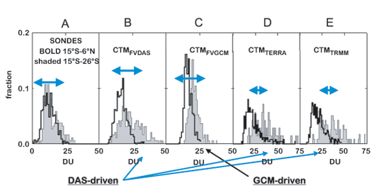Figure 3:PDFs of total ozone, observations and chemical transport model (CTM).  PDFs from DAS-driven show displaced means and spreads that are too wide, whereasGCM-driven PDFs have displaced means with a better half-width.  This shows that there is too much tropical-extratropical mixing in DAS. From Douglass et al. (JGR, 2003). For better resolution, please contact the SPARC Office.

There are a number of points to be made in this figure. First, the winds from the assimilation system in Panel B and the model in Panel C both use the finite-volume dynamics of Lin (2004). Therefore, these experiments are side-by-side comparisons that show the impact of inserting data into the model. Aside from developing a bias, the assimilation system shows much more mixing. As Douglass et al. show, the instantaneous representation of the wind is better in the assimilation, but the transport is worse. This is attributed to the fact that there are consistent biases in the model prediction of the tropical winds and the correction added by the data insertion causes spurious mixing. Tan et al. [2004] investigate the dynamical mechanisms of the mixing in the tropics and the subtropics. Second, the assimilation systems used for Panels D and E have a different assimilation model, and their representation of transport is worse than that from the finite-volume model. This improvement is attributed to the fact that the finite-volume model represents the physics of the atmosphere better, in particular, the representation of the vertical velocity. Third, the results in Panel B show significant improvement compared to the older assimilation systems used in Panels D and E. Older assimilation systems have enough deficiencies that scientists have shied away from doing tropical transport studies. This example demonstrates both the improvements that have been gained in recent years, and indicates that the use of winds from assimilation in transport studies might have fundamental limitations.

Figure 4 (see colour insert IV) is from Schoeberl et al. (2003). The Schoeberl et al. (2003) study is similar in spirit to the Douglass et al. study, but uses Lagrangian trajectories instead of Eulerian advection schemes. This allows Schoeberl et al. (2003) to address, directly, whether or not the spurious mixing revealed in the Douglass et al. (2003) paper is related to the advection scheme. In this figure the results from two completely independent assimilation systems are used; UKMO (United Kingdom Met Office) and DAO (Data Assimilation Office). The DAO system uses the finite-volume dynamical core (labelled DAO) and the finite-volume GCM (labelled GCM). Vertical winds are also calculated two ways, diabatically using the heating rate information from the assimilation system, kinematically, through continuity, using the horizontal winds from the assimilation.

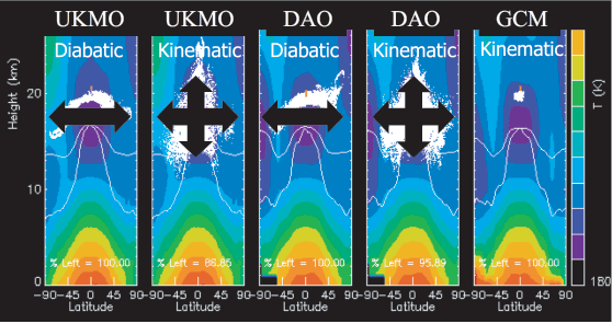Figure 4: Three-dimensional trajectory calculations: The distribution of particles 50 days after the beginning of a back trajectory calculation of parcels initialized at 20 km and the equator.  The lower (upper) thin white line shows the zonal mean tropopause (380 K isentrope).  Zonal mean temperature is indicated by the colour contours and particles are shown as white dots.  Results are from the Met. Office Data Assimilation System (UKMO), the NASA Data Assimilation Office (DAO) analysis, and a GCM.  The Kinematic method shows considerable vertical and horizontal dispersion, while the Diabatic method (using smoothed heating rates) show reduced vertical dispersion.  The GCM shows very little dispersion, regardless of method used, but the assimilated fields are excessively dispersive.  From Schoeberl et al. (2003). For better resolution, please contact the SPARC Office.

The figure shows the impact of the method of calculating the vertical wind using the diabatic information. When the diabatic information is used there is much less transport in the vertical. While this is generally in better agreement with observations and theory, the diabatic winds no longer satisfy mass continuity with the horizontal winds. This points to a self-limiting aspect of using diabatic winds in Eulerian calculations such as the ones of Douglass et al. (2003). The Schoeberl et al. calculations also show that even with the diabatic vertical winds, there remains significant horizontal mixing, which is compressed along isentropic surfaces. The final panel shows that for the simulation, the free-running model, there is much less dispersion, which is in better agreement with both observations and theory. Schoeberl et al. attribute the excess dispersion in the assimilation systems to noise that is introduced by data insertion. (They also note that the finite-volume dynamics is much improved relative to previous generation models.)

TOP

Ozone Assimilation

The last five years have seen the publication of a number of papers on the assimilation of ozone and other constituents. These studies show constant improvement in the state of the art. They demonstrate the importance of having both total column observations as well as high-resolution profile information. Because of this progress, products from ozone assimilation are on the verge of being geophysically interesting. Applications, for example, include improvement of radiative transfer, monitoring of instruments, and providing information useful for estimating tropospheric ozone.

Figure 5 (see colour insert IV) shows an example from an assimilation of ozone data (Wargan et al. 2005). In this example, there are two satellite instruments, the Solar Backscattered Ultraviolet/2 (SBUV) and the Michelson Interferometer for Passive Atmospheric Sounding (MIPAS). SBUV is a nadir sounder and measures very thick layers with the vertical information in the middle and upper stratosphere. MIPAS is a limb sounder with much finer vertical resolution and measurements extending into the lower stratosphere. SBUV also measures total column ozone, which is assimilated in all experiments. The results from three assimilation experiments are shown through comparison with an ozonesonde profile. Ozonesondes were not assimilated into the systems, therefore, these data provide an independent measure of performance.

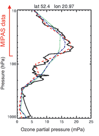Figure 5:Comparison of an individual ozonesonde profile (black line) with three assimilations that use SBUV total column and stratospheric profiles from SBUV (green), SBUV and MIPAS (blue), and MIPAS (red).  Note that the MIPAS assimilation captures the vertical gradients in the lower stratosphere, whereas the using the model and the data captures synoptic variability and spreads MIPAS information. For better resolution, please contact the SPARC Office.

There are several attributes to be noted in Figure 5. The quality of the MIPAS-only (+ SBUV total column) assimilation is the best of those presented. This suggests that the vertical resolution of MIPAS instrument has a large impact. Even though the MIPAS observations are assimilated only above 70 hPa, the assimilation captures the essence of the structure of the ozone profile down to 300 hPa. This indicates that the model information in the lower stratosphere and upper troposphere is geophysically meaningful. Further, the model is effectively distributing information in the horizontal between the satellite profiles. The comparison with the SBUV-only (+ SBUV total column) assimilation shows that the thick-layered information of the SBUV observations, even in combination with the model information, does not represent the ozone peak very well. This impacts the quality of the lower stratospheric analysis as the column is adjusted to represent the constraints of the total ozone observations. Finally, from first principles, the combined SBUV and MIPAS assimilation might be expected to be the best since it has the maximum amount of information. This is not found to be the case, and suggests that the weights of the various error covariances and the use of the observations can be improved. The optimal balance of nadir and limb observations is not straightforward, and these experiments reveal the challenges that need to be addressed when multiple types of instruments are used in data assimilation.

Summary

The question is raised as to whether or not we have reached a limit in the transport and climate problems that can be addressed with assimilated data. Clearly, we have reached a point where the lack of physical consistency is impacting the ability to study the problems at hand. This is true not only in transport studies, but in any studies that require a consistent, closed budget. Furthermore, because of the exquisite sensitivity of data assimilation systems to the input observations, long-term trends strongly reflect changes in the observing system. Improvement in the quality of assimilated data systems is most likely to follow the use of new observations, the reduction of bias, and the development of bias correction techniques. The reduction of bias, and the key to development of assimilated data sets for use in chemistry and climate, will depend on the development of improved physical parameterizations. These improvements should include the ability to directly predict and constrain new observations of the physical processes. Based on recent experience, the details of the assimilation method, i.e. the statistical analysis algorithm, and the improvement of the representation of error covariance are secondary to addressing the problems of bias and physics.

References

Brasseur, G., and S. Solomon, Aeronomy of the Middle Atmosphere, D. Reidel Publishing Company, 452 pp, 1986.

Cohn, S. E., An introduction to estimation theory, J. Met. Soc. Japan, 75 (1B), 257-288, 1997.

Daley, R., Atmospheric Data Analysis, Cambridge University Press, 457 pp, 1991.

Dee, D. P., and A. da Silva, Data assimilation in the presence of forecast bias, Q. J. Roy. Meteor. Soc., 124 (545), 269-295 Part A, 1998.

Dessler, A. E., The Chemistry and Physics of Stratospheric Ozone, Academic Press, 214 pp, 2000.

Douglass, A. R., M. R. Schoeberl, R. B. Rood, and S. Pawson, Evaluation of Transport in the Lower Tropical Stratosphere in a Global Chemistry and Transport Model, J. Geophys. Res., 108, 4259, 2003.

Holton, J. R., An Introduction to Dynamic Meteorology, Elsevier Academic Press, 535 pp, 2004.

Jacobson, M. Z., Fundamentals of Atmospheric Modeling, Cambridge University Press, 672 pp, 1998 - (2nd Ed, to appear, 2005).

Jackman C. H., P. D. Guthrie, and J. A. Kaye, An intercomparison of nitrogen-containing species in Nimbus 7 LIMS and SAMS data, J. Geophys.Res., 92, 995-1008, 1987.

Kistler R. et al., The NCEP-NCAR 50-year Reanalysis: Monthly means CD-ROM and documentation, Bull. Amer. Meteor. Soc. 82, 247-267, 2001.

Lait, L. R., Systematic differences between radiosonde measurements, Geophys. Res. Lett., 29, 1382, 2002.

Lin, S.-J., and Rood, R. B., Multidimensional Flux-Form Semi-Lagrangian Transport Schemes, Mon. Wea. Rev., 124, 2046-2070, 1996.

Lin, S. J., A “vertically Lagrangian” finite-volume dynamical core for global models, Mon. Wea. Rev., 132, 2293-2307, 2004.

Long, C. S., A. J. Miller, H. T. Lee, J. D. Wild, R. C. Przywarty, and D. Hufford, Ultraviolet index forecasts issued by the National Weather Service, Bull. Amer. Meteorol. Soc., 77, 729-748, 1996. Molod, A., H. M. Helfand, and L. L. Takacs, The climatology of parameterized physical processes in the GEOS-1 GCM and their impact on the

GEOS-1 data assimilation system, J. Climate, 9, 764-785, 1996.

Randall, D. A. (Ed.), General Circulation Model Development: Past, Present, and Future, Academic Press, 807 pp, 2000.

Rood, R. B., Numerical advection algorithms and their role in atmospheric transport and chemistry models, Rev. Geophys., 25, 71-100, 1987.

Rood, R. B., D. J. Allen, W. Baker, D. Lamich, and J. A. Kaye, The Use of Assimilated Stratospheric Data in Constituent Transport Calculations, J. Atmos. Sci., 46, 687-701, 1989

Ruhnke, R., C. Weiss; T. Reddmann, and W. Kouker, A comparison of multi-annual CTM calculations using operational and ERA-40 ECMWF analyses, Abstract European Geophysical Society, Nice, 2003.

Schoeberl, M. R., A. R. Douglass, Z. Zhu, and S. Pawson, A comparison of the lower stratospheric age-spectra derived from a general circulation model and two data assimilation systems, J. Geophys. Res., 108, Art. No. 4113, 2003

Simmons, A., Representation of the Stratosphere in ECMWF Operations and ERA-40, in ECMWF/SPARC Workshop on Modelling and Assimilation for the Stratosphere and Tropopause. 23-26 June, 2003.

http://www.ecmwf.int/publications/library/do/ references/list/17123

Stajner, I., L. P. Riishojgaard, and R. B. Rood, The GEOS ozone data assimilation system: Specification of error statistics, Q. J. R. Meteorol. Soc., 127, 1069-1094, 2001.

Stajner, I., N. Winslow, R. B. Rood, and S. Pawson, Monitoring of Observation Errors in the Assimilation of Satellite Ozone Data, J. Geophys. Res., 109, Art. No. D06309, 2004.

Stohl, A., O. R. Cooper, and P. James, A Cautionary Note on the Use of Meteorological Analysis Fields for Quantifying Atmospheric Mixing, J. Atmos. Sci., 61, 1446-1453. 2004.

Swinbank, R., and W. A. Lahoz (Eds.), Data Assimilation for the Earth System, NATO Science Series: IV: Earth and Environmental Sciences, 26, Kluwer, 388 p, 2003.

Tan, W-W., M.A. Geller, S. Pawson and A. da Silva, A case study of excessive subtropical transport in the stratosphere of a data assimilation system, J. Geophys. Res., 109, 2004.

Wargan, K., I. Stajner, S. Pawson, R. B. Rood, and W. –W. Tan, Assimilation of Ozone Data from the Michelson Interferometer for Passive Atmospheric Sounding, Quart. J. Royal. Met. Soc., to appear, 2005.

TOP