|
Stratospheric Processes And their Role in Climate
|
||||||||
| Home | Initiatives | Organisation | Publications | Meetings | Acronyms and Abbreviations | Useful Links |
![]()
|
Stratospheric Processes And their Role in Climate
|
||||||||
| Home | Initiatives | Organisation | Publications | Meetings | Acronyms and Abbreviations | Useful Links |
![]()
Highlights from the Joint SPARC-IGAC Workshop on Climate-Chemistry Interactions
Giens, France, 02-06 April, 2003
A.R. Ravishankara, NOAA, Boulder, USA (ravi@noaa.gov)
S. Liu, Institute of Earth Science, Taipei Tawain, China (shawliu@earth.sinica.edu.tw )With inputs from I. Bey, K. Carslaw, M. Chipperfield, A. Douglas, D. Hauglustaine, C. Mari, K. Rosenlof, T. Shepherd, and P. Simon
Participants at the “Joint SPARC-IGAC Workshop on Climate-Chemistry Interactions, in Giens, France.
Many agents force Earth's climate. Changes in these agents or forcings can perturb the climate significantly. Atmospheric chemistry plays a critical role in the perturbation of climate by controlling the magnitudes and distributions of a large number of important climate forcing agents. For example, abundances and distributions of methane and ozone depend critically on the atmospheric chemistry. According to IPCC (2001), these two trace gases are the second and third most important greenhouse gases (GHGs) that have increased due to anthropogenic activities since the industrial revolution.
Effects of anthropogenic aerosols on the climate could be even greater, with a potential to cancel the positive radiative forcing of GHGs. Aerosols can alter atmospheric radiation directly by scattering and absorbing radiation. This direct effect depends critically on the chemical composition and mixing state of aerosols. Aerosols can also have an indirect effect via their interactions with clouds by acting as cloud condensation nuclei (CCN). Further, clouds can modify aerosols, their optical properties, their size distributions, and their ability to act as CCN. The indirect effect, which is a strong function of the chemical and physical properties of aerosols, can change clouds and even the hydrological cycle, two pivotal components of the climate system. In fact, atmospheric water vapour, a central link of the hydrological cycle, is by far the most important GHG. Any changes in water vapour due to GHGs and aerosols have a large indirect lever on climate.
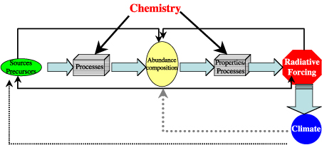
Changes in climate can also affect the atmospheric chemistry significantly. For example, a change in water vapour due to change in temperature can alter the oxidation capacity of the atmosphere. A change in temperature or relative humidity can change the chemical and physical properties of aerosols. Changes in temperature also alter rates of chemical reactions and, thus, composition. These interactions and feedback processes are complex and poorly understood. Therefore, clear understanding of the processes acting in the climate system is essential. Because of their variability in space and time, even the current contributions of short-lived species to radiative forcing cannot be easily evaluated via their atmospheric observations alone. At present, there is a great deal of emphasis on the short-lived species because of the possibility of a quick "return" upon some policy action. Furthermore, these short-lived species are also the "pollutants" that need to be addressed for human health and other concerns. Therefore, clear understanding of the processes that connect emissions (source, precursors) to abundances and the processes that connect the abundances to the climate forcings are essential for an accurate prediction of the future climate and an assessment of the impact of climate change and variations on the earth system (Figure 1).
Figure 1. A schematic depiction of the connections between sources and the atmospheric abundances of radiatively important species and climate. The central role played by processes is indicated in the figure. Indirect effects and feedbacks are also indicated as arrows. Accurate inclusion of these processes, which include chemical, microphysical, radiative, and dynamical processes, is key for understanding climate and for succesfully predicting climate. [From A. Ravishankara]
To assess the current state of our understanding on some of the key issues related to climate-chemistry interactions, a joint SPARC-IGAC workshop was held in Giens, France, on 2-6 April 2003. The specific goal of the meeting was to identify, discuss and prioritise outstanding issues related to the interactions between climate and chemistry that could be attacked jointly by the two research communities. SPARC is a project of the WCRP and IGAC (International Global Atmospheric Chemistry) is a core project of the International Geosphere-Biosphere Program (IGBP).
A. R. Ravishankara and S. Liu, the co-organizers of the joint initiative between SPARC and IGAC, co-chaired the workshop. Other members of the organizing committee were U. Platt , A. O'Neill, T. Bates, S. Fuzzi, and C. Granier. The excellent local organization for the meeting was provided by C. Michaut of the SPARC Office. The meeting went extremely smoothly because C. Michaut (SPARC), C. Burgdorf (NOAA) and K. Thompson (Computer Sciences Corporation) handled the logistic extremely well.
The workshop was divided into five main sessions (Table 1), each with a speaker who summarized the issues pertaining to that session. The talk was followed by short presentations and discussions. The chair of each session organized the discussions and two rapporteurs summarized the findings from the session. In the last session of the workshop, the rapporteurs (with help from the session chairs) summarized the findings to the attendees. The rapporteurs' presentations were followed by further discussion. After the workshop, the rapporteurs (with help from the chairs and other key participants, when necessary) summarized the findings in writing. This written summary is the basis for the highlights given below and will also serve as an input for the white paper that will be generated in 2003.
Table 1. Details of the sessions at the Giens workshop
Session 1 - Aerosols, chemistry, and climate K. Carslaw, P. Quinn T. Bates F. Dentener Session 2 - Water vapour and clouds C. Mari, K. Rosenlof T. Peter U. Lohmann Session 3 - Lower stratospheric ozone and its changes M. Chipperfield, P. Simon U. Platt J. Pyle Session 4 - Tropospheric ozone and other Chemically Active Greenhouse Gases (CAGGs) D. Hauglustaine, I. Bey S. Liu D. Derwent Session 5 - Stratosphere-troposphere coupling T. Shepherd, A. Douglass A. O'Neill R. Rood Session 6 - Final Summary Session All participants Many major issues related to climate and chemistry in general, and climate-chemistry interactions in particular, were discussed. Special attention was paid to identifying uncertainties. All discussions and presentations are summarized in the rapporteurs' report, which will be available at a later date. A few highlights of the workshop are given below to indicate some of the main issues and uncertainties. This is not a comprehensive list, nor is it prioritised at this time; but it serves to give a flavour of the workshop proceedings.
Aerosols, Chemistry, and Climate
Involvement of aerosols in climate, as well as their special role in coupling chemistry with climate, centres around the following issues: (1) transformation and aging processes that affect aerosol composition and properties; (2) chemical processes that determine the global distribution of various aerosols; (3) the radiative impact of aerosols as a function of their chemical composition; (4) the interactions between aerosols and clouds and how they are determined and altered by chemical processes; (5) the role of aerosols in altering the chemical composition of the atmosphere via heterogeneous and multiphase reactions in/on aerosols; and (6) the response of the climate to changes in aerosol abundance and properties.
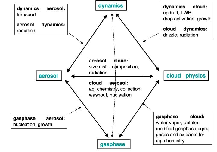
Here we give two examples of the kinds of issues that were discussed. (a) The regional/local nature of the aerosol abundance, properties, and hence their forcings requires calculating these forcings and impacts using very high-resolution models. The global impact can be accurately assessed only after calculating them using high-resolution models. Further, the impacts of climate change due to aerosols will be felt on a regional basis and, hence, understanding them on a regional (smaller) scale is essential. For example, even though the radiative forcing due to long-lived GHGs is longitudinally symmetric, the forcing due to aerosols is very inhomogeneous (see Figures in the IPCC Third Assessment Report). Further, the cooling by sulfate and warming by carbonaceous aerosols are spatially inhomogeneous and do not overlap. So, there will be a very large amount of spatial structure attributed to aerosol forcing. Even on a global scale, the influences can be isolated to some regions, as in the case of cirrus clouds and its primary forcing being in the upper troposphere (UT). The impacts of aerosols in changing the tropospheric composition can also be regional in scale. For example, the interesting and important tropospheric halogen chemistry shown by phenomenon such as the "bromine explosion" in the Arctic is regional and seasonal. Similarly, the impacts can be regional as in the case of the changes due to aerosol emissions by aircraft in the UT/LS. (b) The indirect effects of aerosols are complex processes involving interactions between aerosols, dynamics, cloud microphysics and both gas and heterogeneous phase chemistry. It demands a coupled high-resolution model that incorporates all the above pathways for changes. Figure 2 exemplifies this coupled nature of the indirect effect and the various connections that need to be considered to assess this effect.
Figure 2. The interconnections between various types of processes that need to be included in assessing the direct and indirect effects of aerosols on climate, especially the indirect effect of aerosols arising from their influence on clouds. [From G. Feingold]
There are some commonalities between aerosols and tropospheric ozone (discussed in the session 4 on Tropospheric Ozone and other CAGGs. Both tropospheric ozone and aerosols are climatically and chemically important constituents, both are important in the context of public health, both are short-lived (and thus lead to regional scale forcings), and both are being altered by anthropogenic influences. Also while the impact of long-lived GHGs, which are reasonably well mixed in the atmosphere, is generally well constrained, aerosols and ozone have relatively short lifetimes and their radiative impact is still highly uncertain. The difficulties in incorporating the processes that affect aerosol and ozone abundance in global climate models arise from the high spatial scale resolutions that are needed and the poor state of our understanding of many of these processes. Examples of the spatial variability were also discussed in session 4.
Water Vapour and Clouds
Water vapour is a major climate gas by itself. However, its ability to magnify the contributions of other forcing agents heightens its role. Because water vapour is present in all three of its phases in the atmosphere, it poses a formidable challenge. Water interacts with radiation, changes properties of other forcing agents, provides an important pathway for energy transport and alters the dynamics of the atmosphere. Lastly, water is one of the most important variables of direct concern to life on Earth. Changes in its available amounts, physical state and rate of precipitation are some of the most important predictions needed from climate models. To do so, the climate models have to accurately represent the role of water in the climate system.
The major issues from the point view of global climate systems were noted and discussed: (1) the observation of increases of relative humidity with altitude in the UT; (2) the importance of including water vapour feedback in climate modelling; (3) hemispheric differences in water vapour; (4) homogeneous and heterogeneous freezing of water and their impacts; (5) water vapour trends in the troposphere and the stratosphere; (6) chemistry in clouds.
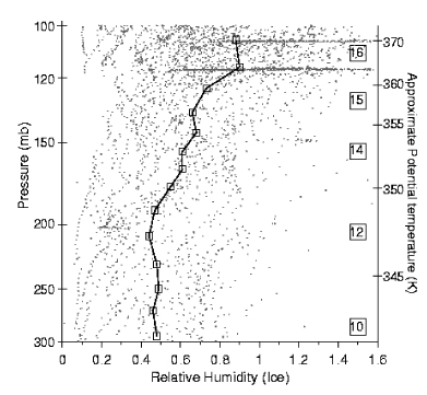
Two examples of the types of questions that were brought up for discussions in this session are given here. (a) What mechanism actually controls the humidity of the UT and the stratosphere and what processes control the long-term trends in water vapour? Figure 3 captures the variation of relative humidity as a function of altitude and clearly shows that often there is vapour present with a super saturation greater than unityThe repercussions of and the processes that lead to such profiles were topics of discussions. (b) How do anthropogenic aerosols affect clouds and, hence, radiation? The key to evaluating and understanding the role of anthropogenic emissions is elucidating how anthropogenic aerosols can alter cloud properties, distributions, etc.
Figure 3. Vertical profiles of relative humidity in the troposphere. Clearly, there are instances where the relative humidity is above unity. The presence of RH greater than unity and the consequences of such values to earth's climate is of great interest in climate science. [From I. Folkins et al.]
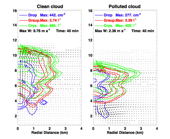
Figure 4 shows the dramatic changes that can occur due to anthropogenic aerosols, which can have different properties of hygroscopicity and cloud condensation capabilities than natural aerosols. Clearly, large-scale changes in water vapour and clouds can be brought about by anthropogenic aerosols and thus have a major impact on climate and precipitation.
Figure 4. The influence of anthropogenic aerosols on cloud properties as computed in a microphysical model shows a significant sensitivity to aerosol loading. Such variations form part of the basis for the current major emphasis on understanding the influence of aerosols on clouds and, thus, on radiation. [From K. Carslaw, Y. Yin]
Tropospheric Ozone and Chemically Active Greenhouse Gases (CAGGs)
A great current policy challenge in tropospheric chemistry is to quantify accurately the future global radiative forcings of climate by methane and ozone. These are the major CAGGs in the troposphere, the others, such as CFCs and N2O, are longer-lived and are removed predominantly in the stratosphere. Recently, concern has also been raised about the possible impact of climate change on tropospheric chemistry and, in turn, on regional air quality in the future. Therefore, variation of the abundances and lifetimes of CAGGs in the future atmosphere is of interest. These variations will depend on the details of the chemistry in the troposphere and, therefore, climate assessments demand an accurate representation of tropospheric chemistry in climate models.
The main questions that need to be addressed in relation to the role of ozone and other CAGGs on climate are: (1) How does tropospheric chemistry affect climate? (2) How does climate change affect tropospheric chemistry? (3) What are the current uncertainties in tropospheric chemistry? (4) What is the role of UT/LS, a key region for climate-chemistry interactions? (5) What type of model is needed to study climate-chemistry interactions? (6) How should one evaluate complex coupled models?
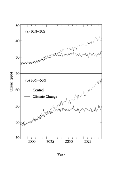
One of the examples that highlight the importance of the above needs is the effect of feedback on calculated future abundance of ozone. The amounts of HOx, and consequently ozone photochemical production and destruction, are highly sensitive to climate changes and variations. This is particularly true for HOx because of the large changes in the abundance of H2O due to climate change. Figure 5 shows the ozone abundances calculated using the STOCHEM model for a future climate and for today's climate. These changes arise primarily due to changes in HOx brought about by climate change. Such interactions between climate change and changes in the abundances of tropospheric species need to be quantified and compared among models and to other processes as changes in dynamics and weather patterns occur due to changes in climate forcing.
Figure 5. Abundances of ozone calculated for equatorial region (panel a) and extratropics (panel b) from the STOCHEM model where the climate is assumed to be invariant with time (control run, dashed line) and where climate changes are included (solid line). These differences arise primarily because of changes in HOx abundances between the control runs calculations where climate changes with time. [From Johnson et al.]
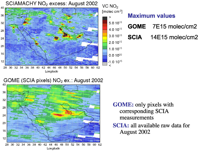
Another example is the resolution dependence of measured and calculated abundances of species responsible for the production or destruction of O3 in the troposphere. Figure 6 shows the measured amounts of NO2 from two satellites with two different resolutions. Clearly, the satellite with the higher resolution shows larger peak amounts in NO2. Because ozone abundances are non-linearly dependent on NOx (= NO + NO2) abundance, such differences due to spatial variations will lead to differences in the calculated concentrations of ozone. Resolution is an issue not only for modelling, but also for emissions and measurements of short-lived atmospheric species, such as ozone and aerosols.
Figure 6. The integrated column abundances of NO2 for the same geographical region and same time from two satellites with differing horizontal resolutions. The lower resolution GOME satellite yields smaller peak column abundances than the higher resolution SCIAMACHY satellite. Since the net ozone production is non-linearly dependent on NOx amounts, these two column abundances would lead to different ozone production rates. These pictures emphasize the need for high resolution atmospheric data and modeling in climate studies. [From J.P. Burrows]
The horizontal and vertical resolutions needed in future global models are certainly important issues to be considered. High resolution is required in source regions to provide a better representation of surface emissions, to account for non-linear effects in atmospheric chemistry and to better represent sub-grid scale processes, such as convection or boundary layer mixing. Such high resolution is also crucial for many other issues.
Lower stratospheric ozone and its changes
Ozone in the lower stratosphere (LS) influences climate and vice-versa. Changes in LS O3 will affect tropospheric climate (as well as LS climate) and climate change will affect LS O3. As LS O3 is partly controlled by chemical processes and partly by dynamics (which is again influenced by the chemical composition of the atmosphere), atmospheric chemistry and climate change are intricately linked together. Therefore, climate change models (i.e., GCMs) should include a realistic description of LS O3, and models aiming to simulate the future composition of the stratosphere should include climate change. The major issues involved in the two-way coupling between chemistry and climate from the perspective of the LS are: (1) transport to the LS, (2) modelling of LS ozone, (3) remote effect of mid-stratosphere changes, and (4) uncertainties due to GCMs.
Source gases (pollutants) reaching the stratosphere are believed to enter mainly at the tropical tropopause. The details of this transport are not fully understood (e.g. the role of the TTL and the processes that take place in this region are major sources of uncertainty). Even though detailed understanding of this region is not critical for long-lived pollutants (e.g. CFCs), what happens in this region is critical for short-lived source gases (e.g. bromine/iodine species). Therefore, we must understand the role of convection/TTL in transporting species to the stratosphere and how it may change in the future (see session on Stratosphere-Troposphere Interactions). In addition to the TTL, the wave driving and chemistry in the troposphere will affect how much and what species reach the stratosphere from the troposphere.
Ozone is chemically long-lived in the LS and its abundance is controlled by both dynamics and relatively slow chemistry (outside of the polar regions in the spring). Both gas-phase and heterogeneous chemistry are important under these cold conditions. We need to improve our understanding of the gas-phase chemistry at low temperature, the surfaces present in the LS/lowermost stratosphere, the heterogeneous chemistry that occurs on these surfaces and the transport for accurately describing LS O3. Stratospheric O3 is expected to increase (‘recover’) as the stratospheric halogen loading declines. Stratospheric cooling is expected to increase mid-stratospheric O3. LS ozone may also increase, but the situation here is more complicated and harder to predict. Increased stratospheric ozone will reduce the UV flux and may decrease tropospheric OH. Therefore, coupled chemistry/climate change calculations must include important feedbacks and extend the model domain high enough to cover the important processes.
In addition to uncertainties in the understanding of processes, there are some major issues related to models. Predictions of future changes in the atmospheric chemical composition will necessarily make use of meteorological forcing fields (temperature, winds, water vapour, convective fluxes, etc.) from GCM simulations. It is therefore of vital importance to have a clear idea of the ability of those GCMs to predict with reasonable accuracy the future climate changes.
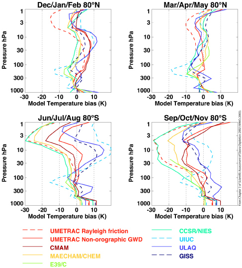
Examples of key model-related issues are temperature biases in the models and the resultant effects on processes in the LS, especially those that depend non-linearly on temperature and/or have threshold temperatures for initiation of certain processes. The modelling calculations carried out so far show that significant biases exist in most models: for instance, temperature biases in the LS can reach several K, which is known to have a strong potential impact on high latitude winter ozone loss, specially in the Arctic. Such biases are shown in Figure 7.
Figure 7. Calculated vertical profiles of temperatures from different climate models. The large differences in calculated temperatures lead to differing abundances of species and ozone changes. [From J. Austin et al.]
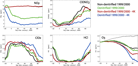
These biases will affect the amount of chemical loss calculated through, for example, different amounts of denitrification, which is shown in Figure 8. Mean meridional transport can also be largely different from model to model, either because of physical reasons (gravity waves, convection, etc., leading to different Brewer-Dobson circulations) or simply because of numerical reasons (location of the upper boundary of the model, numerical algorithms, etc.). Major problems also appear in the models’ water vapour fields, especially in the UT/LS region. The consequences of differing temperatures lead to different predictions.
Figure 8. Evolution of different chemical species (noted in the panels) in the Arctic LS calculated with a 3D-model and using different assumptions of the extent of denitrification produced for various temperatures. [From S. Davies, University of Leeds].
Stratosphere-troposphere coupling
The classical picture of stratospheric transport, in which material enters the stratosphere in the tropics, is transported poleward and downward and finally exits the stratosphere at middle and high latitudes, was proposed to explain observations of stratospheric water vapour [Brewer, 1949] and ozone [Dobson, 1956]. This conceptual model has since been refined but not drastically altered. Holton et al. (1995) pointed out that this Brewer-Dobson circulation is controlled by stratospheric wave drag (quantified by the Eliassen-Palm flux divergence), sometimes coined the “extratropical pump”, with the circulation at any level being controlled by the wave drag above that level. However, the wave drag can be difficult to compute accurately and it is common to diagnose the mean circulation from the diabatic heating. It is possible to estimate the net mass flux across a given isentropic surface from the diabatic heating (for example, the 380 K potential temperature surface, which is nearly coincident with the tropical tropopause and which marks the upper boundary of the lowermost stratosphere). On the other hand, transport of material along isentropic surfaces, such as that between the tropical UT and the lowermost stratosphere, is more difficult to quantify - especially the net transport of a given species that results from the two-way mixing. Observations show that the composition of the lowermost stratosphere varies with season, and suggest a seasonal dependence in the balance between the downward transport of air of stratospheric character and the horizontal transport of air of UT character. For any time period, the integrated mass flux to the troposphere at middle and high latitudes is the sum of the mass flux across the 380 K potential temperature surface, the net mass transported between the tropical UT and the lowermost stratosphere, plus (minus) the mass decrease (increase) of the lowermost stratosphere [Appenzeller et al., 1996]. The first quantity is straightforward to compute, but the last two quantities are sensitive to small-scale processes, including synoptic-scale disturbances and convection.
There are many issues and uncertainties in the stratosphere-troposphere interactions that need to be addressed to have an accurate climate model that couples chemistry and climate. They include: (1) dynamical coupling, (2) tropical stratosphere-troposphere exchange, the TTL, and dehydration, (3) extra-tropics and stratosphere-to-troposphere flux, (4) extra-tropics and troposphere-to-stratosphere flux, and (5) upscaling our knowledge/information, namely to link what we learn from case studies to the representation of various processes in global models, to determine global budgets and to understand their contribution to global change.
Because of these uncertainties, the model range for the O3 flux from the stratosphere to the troposphere, shown in Table 2, is too high. There are not sufficient observational constraints to judge these models. In addition to the net mass flux, it is important to understand longitudinal variations in the stratosphere-to-troposphere flux, as these will be important for short-lived species and for tropospheric chemistry. Such fluxes need to be assessed not only for today's atmosphere, but also for an atmosphere of the future with a different climate. Measurements are needed to examine both seasonal and spatial variability of species in the lowermost stratosphere, using a range of tracers with a spectrum of lifetimes.
Table 2. Tropospheric O3 budgets for circa 1990 conditions from a sample of global 3D-CTMs
CTM-ref MATCH-a MATCH-MPIC-b TM3-c TM3-d HARVARD-e GCTM-f UlO-g ECHAM4-h MOZART-i STOCHEM-j KNMI-k UCl-I NEW Synoz-m
GISS II GISS II’ Oslo/EC These budgets do not always balance exactly (STE+P-L=SURF)
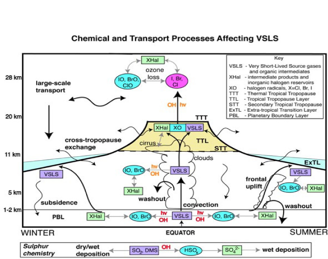
The classical picture of the stratosphere-troposphere coupling has evolved over the last few years. The modification of the Holton diagram for the assessment of the transport of short-lived species to the stratosphere is shown in Figure 9. Such developments and "tuning" are essential for a good description of processes that are important for climate-chemistry coupling.
Figure 9. A schematic representation of the chemical and transport processes that influence stratosphere-trosposphere interactions. In particular, these processes have a significant influence on the TTL region. [From P. Haynes, R. A. Cox, and K. Law]
Summary
These highlights, along with the details of all the other presentations and discussions, form the basis for assessing the current state of climate-chemistry interactions and recommending the research needed to address the unresolved issues. This task will be taken up by the organizing committee in collaboration with a few members of the scientific community to write and publish a white paper that will be released later this year, with A.R. Ravishankara (SPARC Co-Chair, SSG) and S. Liu (IGAC Co-Chair, SSC) as the lead authors.
![]()