|
Stratospheric Processes And their Role in Climate
|
||||||||
| Home | Initiatives | Organisation | Publications | Meetings | Acronyms and Abbreviations | Useful Links |
![]()
|
Stratospheric Processes And their Role in Climate
|
||||||||
| Home | Initiatives | Organisation | Publications | Meetings | Acronyms and Abbreviations | Useful Links |
![]()
UV Index Forecasting Practices around the World
Craig S. Long, NOAA/NCEP, Camp Springs (MD, USA ( Craig.Long@noaa.gov)
Introduction
The forecasting of ultraviolet (UV) radiation at the surface is really the result of separate forecasts of stratospheric ozone, clouds, and eventually aerosols. It was in 1992 when Canada began issuing the first forecasts of UV radiation and actually created the term “UV Index”. Shortly thereafter, many more countries began to issue next day forecasts using simple forecasting techniques. Over the years as the radiative transfer models have become more accurate and the understanding of how other physical conditions like clouds, aerosols, surface albedo and elevation affect UV radiation, the forecast errors of the UV Index have diminished. This article will discuss the latest methods meteorological services are using to forecast the UV Index.
Background
In the summer of 1994 a new international atmospheric parameter was created: the Ultraviolet Index. Until then there were almost as many variations of the UV Index as there were countries giving out this information. The WMO “Meeting of Experts” [WMO, 1994, and WMO, 1997] not only defined what the UV Index was, but also created standards for its forecasting. In 2001 the World Health Organization (WHO) hosted a meeting to further standardize the health messages, exposure categories, and presentation issues dealing with the UV Index [WHO, 2001]. Currently, a few countries have adopted these new standards. Several more are making plans to switch over to these new standards in 2004.
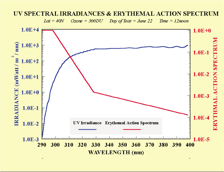
UV Index was defined to be the scaled integral of spectral irradiances between 290 and 400 nm weighted by the CIE erythemal action spectrum [McKinlay and Diffey, 1987]. Figure 1 shows a typical spectrum of irradiances in the 290 to 400 nm range along with the CIE weighting function. Note that the variability of the irradiances is fairly small in the UV-A (320 – 400 nm) part of the spectrum, whereas in the UV-B (280-320 nm) part there are several orders of magnitude changes in the irradiances. Ozone in the stratosphere absorbs all of the incoming UV-C (l<280 nm), some of the shorter UV-B wavelengths, and virtually none of the UV-A wavelengths. As ozone amounts increase (decrease), less (more) UV-B radiation penetrates the ozone layer and reaches the surface.
Figure 1. Spectral irradiances (blue line) derived from an RTM in the UV-B and UV-A wavelengths for clear sky conditions at 40°N, 300 DU of total ozone, on June 22 at solar noon, at sea level with albedo of 5 %. The CIE (erythemal) action spectrum (red line) has greatest weight at the shortest wavelengths.
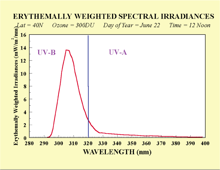
The CIE action spectrum seeks to replicate the average human skin response to UV irradiances. The human skin has evolved to be most sensitive to that part of the UV spectrum, which has the greatest variability due to ozone changes and lesser sensitivity to the part of the UV spectrum that varies the least with ozone changes. The weighted irradiances are shown in Figure 2. Note that the greatest contribution occurs near 310 nm for the described conditions. The peak will vary between a range of 305 and 310 nm for different ozone and solar zenith angle (SZA) conditions. As total ozone decreases (increases) and the SZA decreases (increases), the peak will move to shorter (longer) wavelengths.
Figure 2. Spectral irradiances from Figure 1 weighted by the CIE action spectrum. Integrating these weighted irradiances provides an erythemal dose rate (W/m2). The UV Index is determined by scaling the dose rate by 40.
Integrating these weighted irradiances results in an erythemal dose rate given in units of Watts/m2. The UV Index is then determined by scaling the erythemal dose rate expressed in W/m2 by 40 m2/W resulting in a unitless value that can range from zero at nighttime or in polar night to greater than 15 on top of high mountains in the tropics at solar noon. The greater (lesser) the UV Index, the shorter (longer) the period of time before skin damage will occur. Just how long the time of exposure can be depends upon how much melanin is in your skin and other genetic factors.
Physical Factors affecting UV radiation Forecasting
Radiative Transfer Models determine the Clear-Sky UV radiation
Several physical factors determine how much UV radiation passes through the atmosphere and reaches the surface. These include extraterrestrial solar radiation, total ozone amount, clouds, aerosols, surface elevation and albedo. Most countries use a radiative transfer model (RTM) to determine the clear-sky UV Index inputting some or all of the above parameters (except clouds). Koepke et al. (1998) discuss most of the RTMs used today as part of the European COoperation in the field of Scientific and Technical research (COST-713) action on “UV-B forecasting” (http://www.lamma.rete.toscana.it/uvweb/index.html). In this paper three groups of models are identified: multiple scattering spectral models, fast spectral models and empirical models. In lieu of utilizing the spectral models, empirical relationships can be determined from observed ozone and observed surface UV radiation. For example, Canada utilizes its network of Brewer spectral radiometers to measure the total ozone and UV radiation. Then by using forecast fields from their numerical weather prediction (NWP) model, the next day’s ozone and surface UV amounts are empirically derived. Some countries that have one or multiple Brewers have chosen this way of performing their UV forecasting. The limiting factor with this technique is that the empirical relations have to be tuned to the Brewers used.Total Ozone Source and Forecasting Techniques
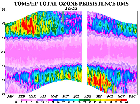
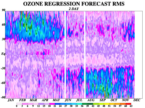
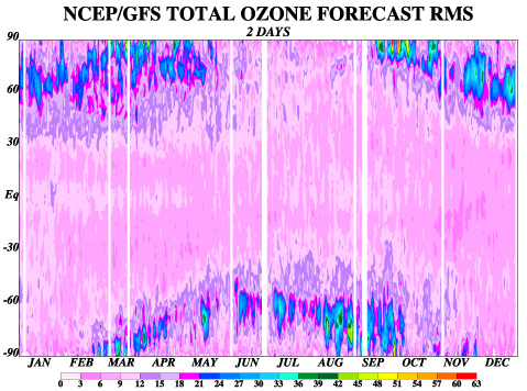
Instead of using ground-based measurements of total ozone, satellite-derived total ozone amounts can be used with the RTMs to determine the UV radiation at the surface. There are four instrument sources of total ozone currently used by the different meteorological services. These are the NASA/Total Ozone Mapping Spectrometer (TOMS), NOAA/Solar Backscatter UltraViolet Instrument (SBUV/2), the ESA/Global Ozone Measurement Experiment (GOME), and the NOAA/TIROS Operational Vertical Sounder (TOVS). The choice of the instrument used will affect the surface UV results by about 5 %. The first three are UV backscattering instruments. The TOVS algorithm uses the 9.7 mm ozone window in the infrared. Comparisons of the TOMS and GOME with surface observations from the Dobson network have shown that the TOMS data are consistently positively biased by about 2 %, whereas the GOME data are negatively biased by about 2 %. The GOME data also show a seasonal variation of this bias. The SBUV/2 has been shown to be positively biased against Dobson observations by 2 %. Comparisons of TOVS and SBUV/2 have consistently shown the TOVS to have a low bias of 2 to 3 % in the tropics and a large positive bias of 3 to 6 % in the winter hemisphere middle latitudes.There are three techniques for making a forecast of total ozone: persistence of the present ozone amounts, utilizing regression statistics between ozone and other meteorological parameters such as geopotential height, temperature, and/or potential vorticity, and lastly assimilation of the ozone data into a NWP model. Figures 3a, 3b, and 3c show the RMS error for over a year’s worth of data utilizing the above three methods. All forecasts are validated against their own “truth”. The figures show that the persistence has the greatest RMS errors. The regression method shows reduced RMS errors, and the assimilated ozone shows the smallest RMS errors.
Figure 3. a) Daily zonal mean RMS errors (DU) obtained by persisting the TOMS total ozone over a 2-day period for the year 2002. b) Daily zonal mean RMS errors (DU) obtained by using a regression method previously used at NCEP to produce a 2-day forecast of ozone. c) Daily zonal mean RMS errors (DU) obtained using the 2-day ozone forecasts from the NCEP/GFS model. Aerosols
The other inputs into the RTM to determine the clear-sky UV Index are determined for the geographic location and day of the year. Next to ozone the most variable parameter influencing the clear-sky UV Index is aerosol content. Aerosols either scatter or absorb UV radiation. The aerosols in the troposphere can be characterized by their optical depth (AOD) and their Single Scattering Albedo (SSA), which is the ratio of the scattered to the total extinction (total extinction = scattered + absorbed). AOD can vary from 0.1 in very clear air to 1.5 in very turbid air. SSA can range from 0.7 to 1.0. As the AOD increases, more UV radiation is scattered and the smaller the SSA becomes, the more UV radiation is absorbed. The AOD and SSA do vary with wavelength. Medium to large AOD can be detected by satellite over the ocean, but is difficult over land due to the variable emissivities of different ground cover and geographic features. Standard AOD, SSA, and aerosol profiles have been developed for different times of the year and source regions (continental, desert, maritime). These standard aerosol parameters are the best that can be done currently until AOD and aerosol profile information can be determined over land by satellite. Then just like ozone it can be assimilated in a NWP scheme to provide forecasts.Elevation
The elevation (or the pressure) of the surface dictates through how much of the atmosphere the direct beam is scattered. The greater the depth of the atmosphere the UV radiation has to be scattered, the lesser the amount reaches the surface. Given the surface elevation the RTM will determine how much more radiation reaches the surface. Generally, UV radiation will increase by about 8 % per kilometre. The RTMs do indicate that the rate per kilometre decreases over the second and third kilometre of elevation gain. Some studies have shown much larger rates of up to 18 % between valley and peak observations. These results did not account for the change in aerosol loading in the atmosphere, which significantly contributes to decreased amounts of UV radiation especially in mountain valleys.Surface Albedo
The albedo of the earth’s surface is nearly black in the UV-B part of the spectrum with values typically between 3 and 5 %. So a very small component of the UV radiation is reflected upwards. Even water has a relatively low albedo of 10 %. Sand is brighter at 30 %. But snow is the most reflective surface. A pure fresh snow surface uninterrupted for several miles can have an albedo of 80 %. However such situations are rare in the mid-latitudes. More frequently, the surface is not flat and has vegetation that extends upward beyond the snow surface. These all reduce the albedo to more like 50 % for fresh snow. As snow ages or melts its reflective qualities decrease to a value more like 30 %. Due to snow’s higher albedo, UV conditions on the ski slopes can approach summer conditions.Extraterrestrial Radiation
The RTMs use the irradiances at the top of the atmosphere as detected by the Atlas 3 or the SUSIM instruments. Both are within good agreement of each other. The RTMs will also determine from the day of year what the earth - sun distance ratio is, so that the extraterrestrial solar radiation is adjusted to be greater in January than in July. Along with the day of year, the time of day, the latitude, and the longitude the RTM can determine the SZA. The greater the SZA, the greater the path length through the atmosphere, and the greater the amount of absorption by ozone and scattering by aerosol.RTMs can be computationally expensive if need to run for more than just a few locations. In practice the meteorological services that make forecasts on grids develop Look Up Tables (LUT) based upon different scenarios of ozone amounts, aerosol content, SZA, and snow/no snow albedos. These LUTs are computationally much faster than running the RTM for each grid point. The errors associated with LUTs tend to be smaller than 5 %.
Cloud Effects
The UV Index value that the RTM or empirical method determines is the maximum amount of UV radiation to be expected under “clear sky” conditions. Since the earth is covered 50-60% of the time with clouds, appropriate cloud modification factors (CMF) have been developed by several campaigns noting the attenuation of observed UV radiation in the presence of clouds and using a RTM to determine what the clear sky condition would have been. One of the recommendations coming from the COST 713 action are the CMFs to be used based upon the cloud fraction and the level (low, mid or high) of the clouds. Table 1 shows these recommendations. The table gives mean conditions for cloud level and amount. As cloud amount increases the optical qualities of the clouds can vary dramatically, thus making the RMS error of these recommendations increase.
Table 1. COST 713 suggested cloud modification factors for various cloud amounts and cloud levels.
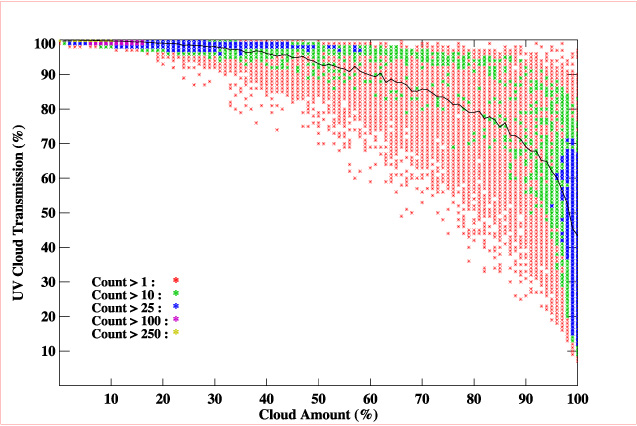
Cloud Level Low (<3 km) Middle (3-7 km) High (>7 km) Cloud parameters coming out of a NWP model usually give the low, mid and high cloud fractions. Information about their optical depths is rarely output. But within the NWP model the shortwave radiation code takes into account the optical properties of clouds as they are parameterized within the model. The Global Forecasting System at NCEP determines the surface flux in discrete bands within the UV-B part of the spectrum with and without the clouds determined by the model. The ratio of the two provides the attenuation in the UV-B wavelengths due to clouds. Figure 4 shows the scatter plot of cloud fraction versus attenuation for one day’s set of NWP model grid points. The mean value is very similar to that suggested by COST 713 and that observed by other campaigns. The more outstanding feature is the large range of values at higher cloud fractions. Validation of these attenuation values needs to be performed. The timing of the clouds is equally as important as the amount of attenuation. With model forecasts being output at a low frequency of every 6 or 3 hours, mean conditions are usually assumed over that period of time. A better cloud output frequency would be every 1 hour. Higher frequencies are limited by the frequency of the radiation package being called within the NWP model and the storage available for the greater amounts of output.
Figure 4. Scatter plot of the ratio of UV band “cloudy sky” and UV band “clear sky” with total cloud amount for each NCEP/GFS model grid point for a single day in the NH mid latitudes (30° – 60°N). The different colour symbols denote the frequency of occurrence. The line is the mean ratio for each cloud amount percent.
Many countries do not have the budget or computer facilities to determine a UV Index forecast. For Europe’s benefit, another action coming out of the COST 713 was that the Deutscher Wetterdienst (DWD) would produce gridded ozone forecasts and UV Index values primarily over Europe. The DWD also produces global gridded fields as well.
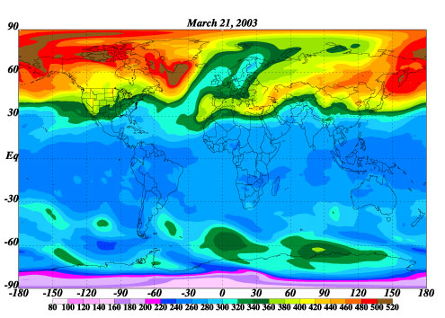
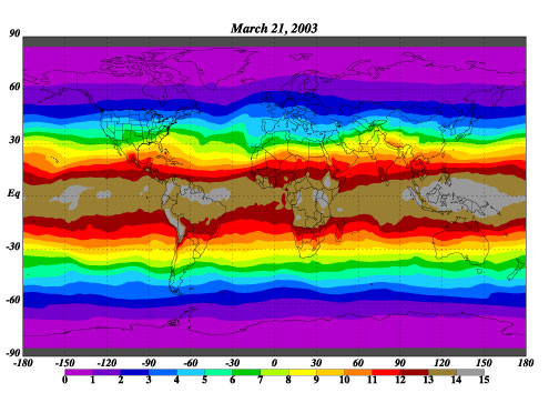
The University of Vienna produces a global clear sky UV Index forecast. These maps are posted on their web page. The U.S. National Weather Service’s NCEP and Australian Bureau of Meteorology (BOM) also generate global forecast grids of ozone and clear sky UV Index values. Figures 5 shows the NCEP/GFS ozone forecast field valid for March 21, 2003 and the resulting clear sky UVI forecast. The NCEP ozone forecast grids are available via anonymous ftp at ftpprd.ncep.noaa.gov/pub/cpc/long/avn_ozone.
Figure 5 a) 2-day total ozone (DU) forecast field generated by the NCEP/GFS model valid for 00Z on March 21, 2003. b) 2-day clear sky UV Index forecast field valid for solar noon at all longitudes on March 21, 2003. Noontime UV Index values were generated from the total ozone forecast fields like that shown in Figure 5a but for all hours of March 21, 2003.
Inquiry results
Table 2 lists the current thirty countries whose weather service or other agency provides some form of a UV Index forecast. These include almost all the countries of Europe, the U.S., Canada, Taiwan, and Israel in the NH. Australia, New Zealand, Brazil, Argentina, Chile, and South Africa are the only countries from the SH to produce UV Index forecasts. Notable exceptions are mainland China, India, and Russia. There are also several other cities or countries that report observed UV Index values. All weather services follow the WMO standard of producing a 1-day forecast for solar noon either for the entire country or for selected cities. A few weather services provide multi-day forecasts. About half of the weather services provide just a clear sky forecast while the rest do incorporate cloud conditions into their forecasts. Some weather services also provide the expected UV Indices at other hours of the day. All but the three that use empirical relationships use a RTM actively or LUT based upon RTM results. As expected, weather services of countries where snow would be a factor incorporate it into their forecasts. Only one weather service (South Africa) uses persisting ozone amounts due to its tropical location. All the other weather services use ozone forecasts from model assimilations or statistical regressions. Those making statistical regressions most commonly use TOMS, a few use GOME, and one uses TOVS ozone data. Those using the ozone forecasts from NCEP will be using the assimilated SBUV/2 data. The BOM assimilates TOVS ozone data. The KNMI assimilates GOME ozone data. And the DWD assimilates both GOME and SBUV/2 ozone data. At least three European weather services make use of the DWD ozone and UV Index forecast fields. Four weather services use NCEP ozone forecast fields.
Table 2. Current UV Index web pages.
The Future of UV Index Forecasts
As stated in the beginning of this article, UV forecasting is the combination of ozone, cloud and aerosol forecasting. Improvements in these three fields will improve tomorrow’s UV forecast as well as extend the range of reliable forecasts out to several days. Reliable ozone forecasts can be received right now from a number of the world’s leading forecast centres. Clouds affect other products besides the UV Index, so weather services that run NWP models will constantly be trying to improve their cloud schemes. The future of aerosol forecasts is dependent upon the ability to detect aerosols over land via satellite and determine its vertical distribution. Once available, aerosol parameters can be assimilated into NWP models and forecasted.
Changes will be forthcoming in the health aspects of the UV Index. A fact sheet [WHO, 2002] about these new standards is now available on-line. It is the WHO’s wish that all countries which issue a UV Index forecast adopt these new health related standards.
Conclusions
To date approximately 30 countries are producing UV Index forecasts. There are notable exceptions making up a substantial fraction of the world’s population. The models and needed information for making more accurate UV Index forecast have dramatically improved over the past ten years. Ozone forecasting techniques have improved greatly with the assimilation of ozone into NWP models. Cloud forecasting is more difficult as NWP models must forecast the levels, amounts and timing of the clouds. A better product may be for the model to output the total cloud attenuation in the UV part of the shortwave radiation. Aerosols are still parameterized from surface observations and climatologies as satellite aerosol observations over land are still sometime away. Albedo and elevation effects have been studied sufficiently to provide good parameterizations in RTMs. Alternatively, empirical relationships based upon surface observations of ozone and UV amounts provide good results for specific geographical domains.
Validation of the UV Index forecasts was not discussed in this article. It is a vital subject that provides direct feedback to all the components of UV forecasting. To do the subject justice would require another complete article.
References
Koepke, P., and 23 co-authors, 1998, Comparison of models used for UV Index calculations, Photchem. Photobio., 67, pp 657-662.
McKinley, A.F. and B.L. Diffey, 1987, A reference action spectrum for ultraviolet induced erythema in human skin, CIE Journal, pp 17-22,.
WHO, 2002, Global Solar UV Index, A practical guide. Fact Sheet 271, http://www.who.int/mediacentre/factsheet/who271/en/index.html
WMO, 1997, Report on the WMO-WHO meeting of experts on standardization of UV Indices and their dissemination to the public, WMO GAW No 127.
WMO, 1994, Report on the WMO meeting of experts on UV-B measurements, data quality and standardization of UV Indices, WMO GAW No 95.
![]()