S P A R C Stratospheric Processes And their Role in Climate A project of the World Climate Research Programme Home Initiatives Organisation Publications Meetings Acronyms and Abbreviations Useful Links

EuroSPICE: The European Project on Stratospheric Processes and their Influence on Climate and the Environment - Description and brief Highlights

John Austin (john.austin@metoffice.com) and Neal Butchart, U.K. Meteorological Office (UKMO), UK
C. Claud and C. Cagnazzo, Laboratoire de Météorologie Dynamique (LMD), France
A. Hauchecorne and J. Hampson, Service d'Aéronomie (CNRS-SA), France
J. Kaurola, J. Damski and L. Tholix, Finnish Meteorological Institute (FMI), Finland
U. Langematz, P. Mieth, K. Nissen and L. Grenfell, Freie Universität Berlin (FUB), Germany
W. Lahoz and S. Hare, University of Reading (UR), UK
P. Canziani, University of Buenos Aires (UBA), Argentina

1. Introduction

EuroSPICE was composed to bring together observations and a full range of 3D-dimensional models to improve our understanding of the impacts on the atmosphere of changes in the concentrations of the greenhouse gases (GHGs) and halogens. Europe is strong in these activities and funding under the European Framework 5 umbrella has proved to be a particularly useful way of stimulating collaboration between the research groups, which consisted of the UKMO, LMD, CNRS-SA, FMI, FUB, UR and UBA. Addressing the issue of the impact of the stratosphere on climate was from the beginning a long-term aim of EuroSPICE, and assuming that contract negotiations are successful, this will be continued in the European Framework 6 project SCOUT. EuroSPICE has just a few more months to run and this would seem to be an apposite time to summarise its preliminary results, and we welcome informal discussions on the material.

The work was designed to cover the recent past (1980 to 2000), for which good data coverage exists, and the near future (2000 to 2020) to address issues such as the recovery of stratospheric ozone. The work concentrated on trends in temperature, ozone and surface UV. The major data sources were utilised for this purpose with, where possible, a detailed statistical model employed to determine trends. Model simulations were based around transient climate model simulations, with and without coupled chemistry, supported by 3D- mechanistic and chemical transport models. To provide consistency between the model simulations, the sea surface temperatures (SST) were specified from observations and the concentrations of halogens and the well-mixed greenhouse gases (WMGHGs) were taken from WMO [1999, Chapter 12] and IPCC [1992, Scenario IS92a], respectively. Finally, with the model results now available, the impact of the stratosphere on the troposphere is beginning to be investigated, initially using some basic tropospheric parameters.

2. Past trends

(a) Temperature
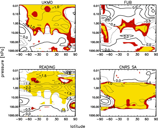
The cooling trend in the stratosphere and warming trend in the troposphere is by now an established feature of the global atmosphere [see e.g. Shine et al., 2003]. This is reproduced by all the models of EuroSPICE. Figure 1 shows the trends determined for transient model simulations. All the models used the same evolution in the concentrations of GHGs and halogens. The UKMO and FUB models are full climate models and used coupled chemistry. The Reading model is a climate model, the Unified Model (UM) is the same version as used by the UK Met. Office, but it doesn't have coupled chemistry. Instead, the ozone trends are specified from the observations determined by Langematz (2000). The CNRS-SA model is a mechanistic model with a lower boundary near the tropopause. Although there are many similarities between these model temperature simulations, differences arise from the different ozone trends as shown in Section 2b.

Figure 1. Annual mean temperature trend for 1980 to 1999 in K/decade simulated by the different models of EuroSPICE. The contour interval is 0.5 K/decade; regions where the trend is significantly different from zero are shaded for the 95 % (red) and 99 % (yellow) confidence levels.

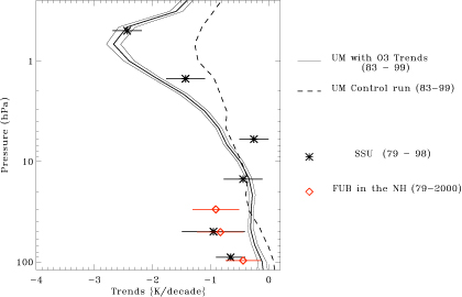
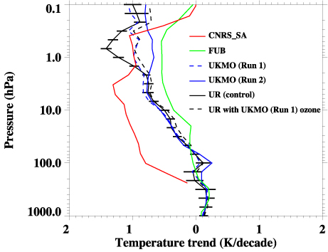
The above model trends have been computed using a simple linear trend model without additional parameters. During EuroSPICE a more detailed statistical analysis has been undertaken of observations from the SSU and MSU satellite data using the AMOUNTS statistical model [Hauchecorne et al., 1991]. Results are shown for the near-global average in Figure 2, together with a sample of the model results shown in Figure 1. Also shown in Figure 2 are the NH temperature trends computed from the FUB analyses using the AMOUNTS model. These results are compared with an additional simulation of the UM in which the GHGs concentrations increase as in the observations but with no trend in ozone, indicated by the broken line in Figure 2. The two UM simulations are significantly different in the upper stratosphere and lower stratosphere (LS), confirming the role of ozone decreases in contributing to the temperature trends in those regions. With the observed ozone trends, the model agrees reasonably with observations through much of the pressure range, except possibly in the LS. These results are very similar to those obtained by Shine et al. (2003) who further suggested that the absence of water vapour trends in the models may be one of the reasons for the remaining discrepancies with observations, particularly in the LS.

Figure 2. Near global average temperature trends from observations and model results. Data for both model and observations are averaged between 70°N and 70°S because of the limited domain of the SSU data. The results of the Unified Model (UM) are the mean for an ensemble of five members. The thick solid line indicates the mean trend calculated by the UM with the ozone trends specified. The 95 % confidence interval is given by the thin solid lines.

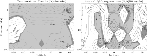
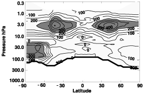
By using the AMOUNTS model, it was possible to investigate the temperature data to separate the various processes affecting variability and to provide, ultimately, a more accurate determination of the underlying trends. The observations were regressed against aerosol, El-Nino Southern Oscillation, Arctic Oscillation, solar variability and the Quasi-Biennial Oscillation (QBO) terms, as well as seasonable terms and the secular trend. As an example, we show in Figure 3 the secular trend and the impact of the QBO on temperature determined from the SSU/MSU data and assuming a phase delay of 7 months. A significant signal is present in the lower and middle stratosphere with opposite phase signals at middle latitudes. The fact that the signal is quite large, comparable with the decadal trend (left panel), implies the need for careful analysis of the model results in the tropics particularly for models such as the UM (used by UKMO and UR), which has a naturally occurring QBO. Without detailed analysis, the significance of the model trends could be lowered by the large interannual variability in the tropics, which might otherwise be interpreted as noise by the statistical trend calculation.

Figure 3. Left panel: Annually averaged temperature trend from the SSU/MSU data. The dark and light shading indicates where the trend is significantly different from zero at the 90 % and 95 % levels, respectively. Right panel: The QBO component of the temperature signal observed by SSU/MSU instruments. The units are K per QBO cycle assuming a 7 month phase lag. The statistical significance of the signal is indicated for the 90 % and 95 % as dark and grey, respectively.

(b) Ozone
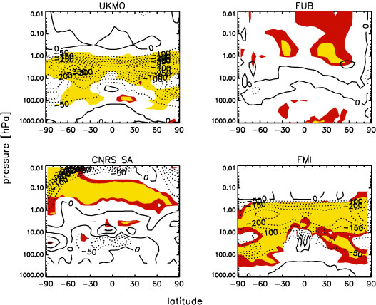
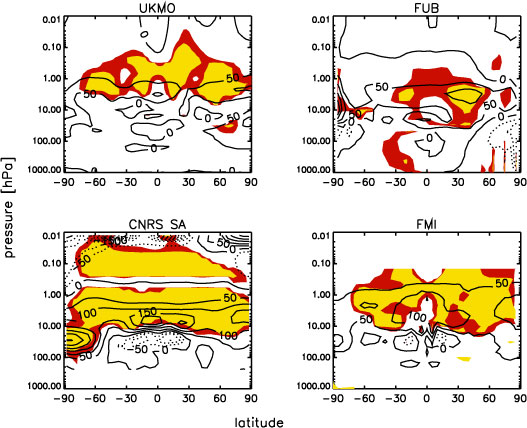
Figure 4 shows the past ozone trends computed by the models of EuroSPICE. An explanation of some of the differences in the model temperature trends is apparent in the large differences in modelled ozone. The models generally fit into two general types: one with large ozone losses in the upper stratosphere (UKMO and FMI) and one with small increases in this region (FUB and CNRS-SA). The first two models also indicate large ozone losses in the polar LS in both hemispheres, consistent with the development of the Antarctic ozone hole and northern spring depletion. These are the very regions affected by halogen chemistry and they are being further investigated by the two models showing ozone increases.

Figure 4. Annual mean ozone trend for 1980 to 1999 in ppbv/decade simulated by the different models of EuroSPICE. The contour interval is 50 ppbv/decade; regions where the trend is significantly different from zero are shaded for the 95 % (red) and 99 % (yellow) confidence levels.

The observations from SAGE (Figure 5) show the high ozone losses expected from the halogen chemistry. At 3 hPa the ozone trends equate to typically 6% per decade with peak values exceeding 8% per decade. The Antarctic ozone hole is clearly visible in the annual mean. Note also the slight increase in ozone at some levels up to 10 hPa over the equator, which is reproduced in the UKMO and FMI models, although it is not statistically significant.

Figure 5. Observed annual average stratospheric ozone trend over the period 1979 to 1997 as a function of latitude and pressure. Data were obtained from Randel and Wu (1999) and the approximate position of the tropopause is indicated by the thick line. Ozone decreases exceeding 250 ppbv per decade are indicated by the shading.

(c) Surface ultraviolet
One of the main aims of EuroSPICE is to clearly establish the relationship between the parameters affecting surface Ultraviolet. While it is clear that ozone trends have been a contributing factor, in principle, aerosol and cloud changes may also have played a role in regions where the UV trend is small. For EuroSPICE we have adopted a simplified way of using climate model output to provide an estimate of the cloud-corrected UV. We have also determined surface UV trends from TOMS, as well as measurements from ground-based instruments over high latitudes in Europe. Figure 6 compares the UV trends from TOMS with those from the UKMO model. Good agreement between model and observations is generally seen, but although the trends at high latitudes are substantial, the large interannual variability increases the uncertainty in the trends. Further analysis of the results indicates that the cloud trend is small. Hence, the cloud-corrected UV levels are dominated by ozone amounts, albeit with the cloud variation increasing the variability and uncertainty in the computed UV trends.

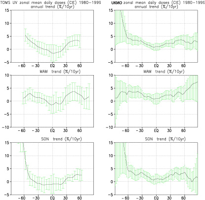
Figure 6. Zonal mean UV trends (% per decade) for TOMS data (left panels) and UKMO model data (right panels) during different seasons (annual, March to May, and Sept. to Nov.). The error bars represent the 95 % confidence range computed using the Student t-test.

3. Future trends

(a) Temperature
The future temperature trends calculated by the models of EuroSPICE are shown in Figure 7.

Figure 7. Simulated globally and annually averaged temperature trends in the models for the period 2000-2019 as a function of pressure. The UR results are shown as a control run with fixed ozone (black line) and a run (black broken line) with ozone from Run 1 of the UKMO simulation. The error bars in the control run indicate the 95 % confidence intervals. For clarity, the uncertainties are not included in the other model simulations but are of similar magnitude.

Comparisons are shown with the UR control run (solid black line with 95% confidence intervals), which assumes constant ozone and projected increases in the concentrations of the WMGHGs. The UR results indicated by the black broken line were calculated using the same underlying climate model but with ozone computed from the first of two runs of the UKMO model. All the UKMO results shown earlier in this article were from Run 2, and they are also shown here for comparison with Run 1.

All the models are generally very close, except for the CNRS SA model which has much higher temperature trends in the lower and middle stratosphere. This model is a mechanistic model with wave amplitudes supplied at the lower boundary, whereas the other models are complete climate models with the same SSTs specified.

(b) Ozone
Figure 8 illustrates the future ozone trends calculated by the models. All the models have a small but statistically significant ozone recovery in at least part of the upper stratosphere, in the region most influenced by halogen chemistry. In the LS, the overall trends are much lower and not statistically significant, suggesting the need for longer integrations before ozone recovery can generally be predicted.

Figure 8. Annually averaged future ozone trends (ppbv/decade) simulated by the models as a function of latitude and pressure. Shading denote the regions where the trend is significantly different from zero at the 95 % (red) and 99 % confidence levels (yellow).

(c) Surface ultraviolet
The small future changes in ozone indicated in Figure 8 and in the total ozone results (not shown) suggest that the future surface UV trends will also be small. This is confirmed in Figure 9, which shows the predicted UV trends for just one of the EuroSPICE models. While in the SH the decrease in UV is not statistically significant during the spring (not shown), in the northern spring the model predicts a significant decrease of about 10% in high latitude UV.

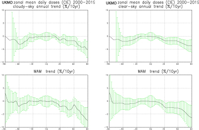
Figure 9. Zonal mean UV trends (% per decade) for UKMO cloudy sky data (left panels) and clear sky data (right panels) for the annual average and the March-May season. The error bars represent the 95 % confidence range computed using the Student t-test.

4. Tropospheric impacts

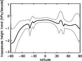
The impact of the stratosphere on the troposphere is one of the major themes of EuroSPICE, but has not so far received full attention because the model simulations have only recently been completed. All the climate model simulations of EuroSPICE show tropospheric warming due to increases in the GHGs concentrations. The uncertainty in the trend, though, arises from the large interannual variability in the troposphere, so that it is difficult to detect a difference in this trend despite a range of stratospheric changes. Other factors which have been examined are cloud cover, precipitation amounts and storm track numbers or intensities with a similarly null result. Figure 10 shows the trend in the tropopause pressure over the full 40 years of a control run with the UM. Most latitudes show a statistically significant decrease in tropopause pressure and in mid-latitude the trend is about –1 hPa/decade, similar to that observed (e.g. Santer et al., 2003). However, so far no significant differences have been detected, suggesting that stratospheric ozone trends have not contributed significantly to tropopause height changes.

Figure 10. Trend in annual mean, zonal mean tropopause pressure in the 1980-2019 control run. The central line shows the trend with 95% confidence intervals delimited to either side.

5. Conclusion

With just a few more months to run, EuroSPICE is nearing its completion. The main highlights so far have been a thorough analysis of temperature data and the completion of simulations with a range of 3-D models from mechanistic to fully coupled chemistry-climate models. Comparisons with observations of ozone and surface UV have also underpinned the project.

Most models captured the broad characteristics of the observed stratospheric temperature trends due to CO₂ increase. Differences existed particularly where models were unable to simulate past ozone trends. Those model trends which agreed with observed ozone trends also generally agreed with past UV trends. For the first time, cloud-corrected UV was computed from the climate model simulations. It emerged, however, that cloud trends were very small and did not affect overall UV trends.

Future simulations indicated only a small recovery in stratospheric ozone by 2020 and, hence, only a slight decrease in future surface UV on this timeframe. Nonetheless, for those models which reproduced the past trends, the future temperature trends were also reduced, particularly in the upper stratosphere, indicating the importance of ozone trends on the temperature.

Although some tropospheric impacts have been investigated, the diagnostics examined so far have not revealed a significant impact of stratospheric change on the troposphere. This may have been related to the model set up, in which SSTs and the concentrations of the WMGHGs were specified. One of the ways that stratosphere-troposphere interaction might be important is through changes in the Brewer-Dobson circulation [e.g. Butchart and Scaife, 2001]. This could have the effect of changing the concentrations of the halogens and the WMGHGs in the atmosphere with consequences for the climate model radiative heating rates.

In the future, further analysis of the model results will take place, to investigate some of the remaining details. There would also likely be opportunities, under European Framework 6, for further model comparisons to take place with the results already obtained. Simulations are also becoming available from countries outside Europe, as illustrated in WMO (2003, Chapter 3) and Austin et al. (2003), which point to a need for broader international collaboration in chemistry-climate coupling. This process is indeed well under way with for example the workshop on `Process-orientated validation of coupled chemistry-climate models' to be held in Garmisch-Partenkirchen in November 2003.

References

Austin, J. et al., Uncertainties and assessments of chemistry-climate models of the stratosphere, Atmos. Chem. Phys., 3, 1-27, 2003.

Butchart, N., and Scaife, A.A., Removal of chlorofluorocarbons by increased mass exchange between the stratosphere and troposphere in a changing climate, Nature, 410, 799-802, 2001.

Hauchecorne, A. et al., Climatology and trends of the mid- atmospheric temperature (33-87 km) as seen by Rayleigh lidar over the south of France, J. Geophys. Res.,96, 15297-15309, 1991.

IPCC, Intergovernmental Panel on Climate Change, Climate change: the supplementary report to the IPCC scientific assessment, ed. J.T. Houghton, B.A. Callander, and S.K. Varney, Cambridge University Press, Cambridge, UK, 1992.

Langematz, U., An estimate of the impact of observed ozone losses on stratospheric temperatures, Geophys. Res. Lett., 27, 2077-2080, 2000.

Randel, W.J. and Wu, F., A stratospheric ozone data set for global modeling studies. Geophys. Res. Lett., 26, 3089-3092, 1999.

Santer, B.D. et al., Behaviour of tropopause height and atmospheric temperature in models, reanalyses and observations. Part I: decadal changes, J. Geophys. Res., In press, 2003.

Shine, K.P. et al., A comparison of model-predicted trends in stratospheric temperatures, Q. J. R. Meteorol. Soc., 129, 1565-1588, 2003.

WMO, Scientific Assessment of Ozone depletion: 1998, WMO Gobal Ozone Research and Monitoring Project, Report No. 44, Geneva, Switzerland, 1999.

WMO, Scientific Assessment of Ozone depletion: 2002, WMO Gobal Ozone Research and Monitoring Project, Report No. 47, Geneva, Switzerland, 2003.