 |
Stratospheric Processes And their Role in Climate
|
||||||||
| Home | Initiatives | Organisation | Publications | Meetings | Acronyms and Abbreviations | Useful Links |
![]()
 |
Stratospheric Processes And their Role in Climate
|
||||||||
| Home | Initiatives | Organisation | Publications | Meetings | Acronyms and Abbreviations | Useful Links |
![]()
Time variations of the atmospheric state have two periodic components known as a diurnal cycle and an annual cycle, which are responses to the periodic variations of the external forcings due to the earth's rotation and revolution, respectively. Intraseasonal and interannual variations are defined as deviations from the periodic annual response; generally the intraseasonal variation means low-frequency variation with week-to-week or month-to-month time scales, while the interannual one means year-to-year variation. Some part of these variations is a response to the time variations of the external forcings or boundary conditions of the atmospheric system, while the rest is generated internally within the system. Well known natural forcings with interannual time scales are the 11-year solar cycle, irregular and intermittent eruptions of volcanoes, and interannual variations of sea-surface and land-surface conditions (e.g., temperature, roughness, snow/ice, ...), although the last ones should be considered as internal variation of the coupled system of the atmosphere, ocean and land. The Quasi-Biennial Oscillation (QBO) of the zonal mean zonal flow in the equatorial stratosphere, which is basically caused by the interaction between the mean zonal flow and equatorial waves propagated from the troposphere, could be considered as variation of a lateral boundary of the mid-latitude stratosphere. In addition to these natural forcings, there are some anthropogenic forcings such as the increases of greenhouse gases, aerosols, chemical constituents related to the stratospheric ozone decrease, or something else. Responses to these anthropogenic forcings are usually called "trends". On the other hand, external forcings are not so significant in the intraseasonal time scales; fundamentally intraseasonal variation is considered as a result of internal processes that may exist even under constant external conditions. Such variation may be a linear periodic oscillation or non-linear variation (periodic, quasi-periodic or chaotic) produced in the atmospheric system. These time variations can be classified systematically with some simple models (Yoden, 1997).
Figure 1 shows an example of the variations in the polar stratosphere; daily temperature at the North Pole (a) has large intraseasonal and interannual variability in winter and early spring, while large variability at the South Pole is seen in spring (c). Large fluctuations at the North Pole are direct results of the occurrence of stratospheric sudden warming (SSW) event, which is associated with a rapid breakdown of the polar vortex from a cold, strong and undisturbed state to another warm, weak and disturbed one. The difference between the two hemispheres is quite noticeable. These intraseasonal and interannual variations are also seen in the monthly mean temperature data. In the equatorial lower stratosphere, the QBO signal is dominant in the original time series of temperature, but the annual component is also discernible in Figure 1 (b); the low temperature in northern winter can be understood as a result of adiabatic cooling due to the stronger upward motion associated with the wave-induced meridional circulation in the northern hemisphere (NH).
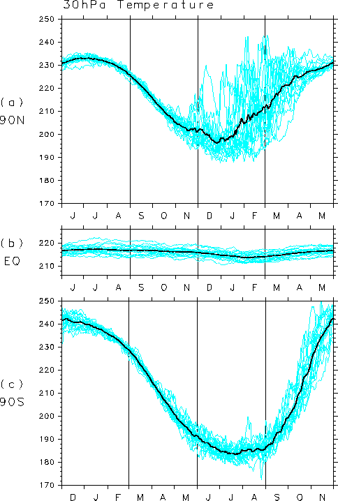
Figure 1: Seasonal variation of daily temperature at 30 hPa at the North Pole (a), the equator (b) and the South Pole (c) drawn with NCEP/NCAR re-analysis data for 1979-1997. Thick black line is the 19-year average for each calendar day.
We have made some numerical experiments with a hierarchy of models over a decade, in order to understand intraseasonal and interannual variations in the polar stratosphere and their dynamical linkage to the troposphere. The importance of a balanced attack with a hierarchy of numerical models was pointed out by Hoskins (1983) a long time ago, and his advocacy has much influenced our experimentation.
Numerical models can be divided into three classes based on their complexity or degrees of freedom (number of dependent variables after spatial discretisation). In the past, only simple low-order models (LOMs) with 100-2 degrees of freedom could be used in parameter sweep experiments due to the limitation of computing resources. We have to be careful with spurious results due to severe truncations in the spatial discretisation, but LOMs are still useful for conceptual description or illustration of the basic dynamics with limited components. Nowadays it becomes possible to use full dynamical models with 104-6 degrees of freedom for parameter sweep experiments. We call them mechanistic circulation models (MCMs). Some idealisation of physical processes in these models helps us to understand the essential dynamics. We do not need to worry about the truncation effect. For quantitative arguments, more complex general circulation models (GCMs) with 104-8 degrees of freedom are necessary, in which sophisticated physical parameterisation schemes should be adopted. However, parameter sweep experiment with full GCMs is still limited even in the most advanced computational environment.
Some simplified models on the interaction between the zonal mean zonal flow and planetary waves propagated from the troposphere have been developed to study the stratospheric variations including SSW events. Yoden (1987, 1990) discussed the intraseasonal and interannual variability in the stratosphere by using LOM introduced by Holton and Mass (1976, hereafter referred to as HM). The HM model is a highly-truncated spectral model which consists of the zonal mean and a single wave components in a mid-latitude beta-channel. Important external parameters in the HM model are the intensity of the mean zonal flow forcing, dUR/dz, and the wave amplitude at the bottom boundary placed near the tropopause level, hB.
Yoden (1987) showed that multiple stable solutions of a cold/strong polar vortex and another warm/weak one may exist for the same external conditions in a finite range of hB, and discussed a possible application of such concept for understanding the intraseasonal variability of the NH winter stratosphere. Some theoretical models of SSW were reinterpreted with the same framework of the HM model. The essence of Matsuno's (1971) theory is an impulsive initiation of a wave forcing in the troposphere; transient response to the increase of hB for a short time interval may cause a rapid transition from the state of cold/strong polar vortex to the other warm/weak state. Another theory of SSW is the stratospheric vacillation found by HM. They showed the periodic variation of the stratosphere that mimics repeated occurrence of SSW events with a period of 50-100 days may exist even for a time-constant hB. The vacillation is a non-linear internal variation of the mid-latitude stratospheric system with fixed external conditions.
These two theories made a very opposite assumption on the dynamical linkage between the troposphere and the stratosphere. Matsuno (1971) assumed a "slave stratosphere"; the stratospheric variation is caused by the variation of its bottom boundary, that is, the troposphere, without any stratospheric influence on the troposphere. On the other hand, HM assumed an "independent stratosphere" in the time variations; the stratospheric variation is possible for a time-constant bottom boundary condition.
Seasonal and interannual variations of the stratospheric circulation have been studied theoretically with some "independent stratosphere" models. Yoden (1990) varied dUR/dz in the HM model periodically with an annual component to investigate the response to the periodic forcing, but did not obtain any example of interannual variations (i.e., deviations from the periodic annual response). The periodic response, or the seasonal variation is qualitatively different depending on hB, and the difference resembles that of the climatological seasonal march between NH and the Southern Hemisphere (SH); larger hB corresponds to NH. By using similar dynamical conditions in a hemispheric primitive-equation model, Scott and Haynes (1998) found interannual variations even for a periodic annual forcing. The internal interannual variability arises owing to the longer "memory" of the stratospheric flow at low latitudes. A given wind signal at low latitudes is less affected by radiative damping, of which time scale is much shorter than a year, due to the smaller Coriolis parameter. Internal variability due to the longer memory of low latitude winds might have a role in the interannual variability in the real stratosphere.
The stratosphere-only models described in the previous section, either "slave stratosphere" models or "independent stratosphere" ones, assume no downward influence from the stratosphere to the troposphere. However, some recent studies pointed out the coupled variability of the troposphere and the stratosphere with intraseasonal and interannual time scales (see, e.g., Baldwin, 2000; Hartmann et al., 2000); the Arctic Oscillation (AO) is a deep signature of zonally-symmetric seesaw patterns of geopotential height, alternating between the polar region and mid-latitudes, from the surface to the lower stratosphere. Such annular variability of the polar vortex is observed in all seasons in both hemispheres and the troposphere-stratosphere (T-S) coupling is stronger in dynamically active season, namely winter in NH and spring in SH. Downward propagation of the AO signature from the stratosphere to the troposphere was noticed in association with SSW events. It was also pointed out that the propagation route of planetary waves is very sensitive to the annular variations. These studies are indicative of the importance of two-way interactions between the troposphere and the stratosphere.
Recent progress in computing facilities enabled us to make some parameter sweep experiments, similar to those done with LOMs over a decade ago, with three-dimensional MCMs in order to understand the T-S coupled variability. Taguchi et al. (2000) modified an atmospheric GCM by making some simplifications of physical processes; all the moist processes were taken out, the radiation code was replaced by a simple Newtonian heating/cooling scheme, Rayleigh friction was used at the surface, and sinusoidal surface topography was assumed in longitudinal direction with a single zonal wavenumber m = 1 or 2 component. It is a spectral primitive-equation model with 42 vertical levels from the surface to the mesopause and its horizontal resolution is given by a triangular truncation at total wavenumber 21 in spherical harmonics. Thus the model has full dynamical process with 105 degrees of freedom.
Under a purely periodic external condition of annual thermal forcing, 10 runs of 100-year integration were done with different topographic amplitude of 0 m ?h0 ?3000 m (Taguchi and Yoden, 2000a). The relative importance of the planetary waves forced by the topography is studied by such parameter sweep. Figure 2 shows the dependence of temperature variations in the polar stratosphere on h0; if it is equal to zero or a small value, the interannual variation is very small, particularly in winter. The variation becomes large in spring for h0 = 400 - 600 m, which looks like the variation in SH as shown in Figure 1 (c). If h0 is increased further, the variation becomes large in winter. The results for h0 = 700 or 1000 m look like the variation in the NH. Note that the interannual variation in this experiment is caused only by the intraseasonal variations which have a random phase depending on each year.
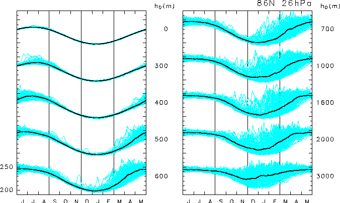
Figure 2: Seasonal variation of daily temperature at 86°N and 26 hPa for 10 runs of 100-year integrations under a purely periodic annual forcing. The topographic amplitude h0 of zonal wavenumber 1 is changed from 0 m to 3000 m as the experimental parameter. Thick black line is the 100-year average for each calendar day.
Taguchi and Yoden (2000b) also made 2 runs of 1000-year integration under the same purely periodic annual forcing. In the millennium integration's, statistically reliable frequency distributions of the monthly-mean polar temperature are obtained (Figure 3). The internally generated interannual variation is very large during winter in the run of h0= 1000 m, while it is large in spring in the run of h0 = 500 m. The distributions for h0 = 1000 m are positively skewed in autumn and bimodal in winter. On the other hand, those for h0 = 500 m have positive skewness for a longer period from autumn to spring and extremely large skewness is found in March. Based on these probability distributions, a question can be raised on the usefulness of ordinary statistical significance tests assuming a Gaussian distribution.
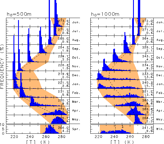
Figure 3: Frequency distributions of the monthly mean polar temperature at p = 2.6 hPa in the two millennium integrations: h0 = 500 m (left) and 1000 m (right). Dashed line denotes the 1000-year mean annual variation of the monthly mean temperature, and orange shade shows the variable range. Averages and standard deviations for the 1000-year data are also written on the right hand side of each panel (top and bottom numbers, respectively). Frequency distributions for a seasonal mean are also displayed in the bottom: spring mean for h0 = 500 m and winter mean for h0 = 1000 m. The downward arrow in the seasonal mean indicates a threshold value for the 200 years of highest temperature.
Figure 4 shows the time series of the deviation of winter-mean polar temperature at p = 2.6 hPa in the millennium integration of h0 = 1000 m, which is made by connecting 10 independent 100-year integration. Here a threshold value is introduced to select the 200 warmest winters denoted by red dots. The occurrence of the warm winters looks like random. In some periods there is no warm winter over decades (e.g., the period around year 410), while warm winters appear frequently in some other periods (e.g., around year 620). To test the randomness, intervals of two consecutive warm winters are examined statistically. Figure 5 shows frequency distribution of the interval of warm winters that is longer than the interval indicated on the abscissa. The cumulated frequency is well fitted by an exponential function A exp(-t/T) as denoted by the broken line with estimated T of 4.5 years. The exponential distribution means that the occurrence of a warm winter itself is described by a Poisson process. That is, the warm winters occur at random from year to year, and preferred periodicity does not exist in the present internal interannual variability.
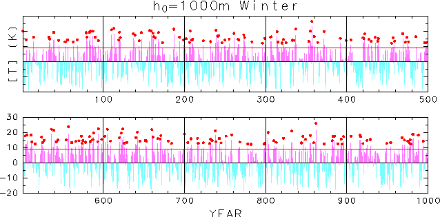
Figure 4: Time series of the deviation of winter-mean polar temperature at p = 2.6 hPa in the millennium integration for h0 = 1000 m, which is made by connecting 10 independent 100-year integrations. The red horizontal line is the threshold value (+ 9.2 K) to select the 200 warmest winters denoted by red dots.
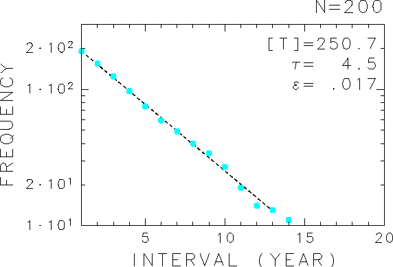
Figure 5: Frequency distribution of intervals of two consecutive warm winters in the millennium integration for h0 = 1000 m. Blue dot shows the frequency (number) of the interval that is longer than the year indicated on the abscissa. The warm winters are defined in Figure 4 as the top 200. The broken line is the best-fit exponential function A exp(-t/T), determined by the least square method. The mean interval T is 4.5 years, and the mean error e =0.017. The scale of e is 1 for one order of frequency.
The warm winters are directly related to the occurrence of SSW events. A lag-correlation (regression) analysis of such intraseasonal variations shows two-way interactions in the T-S coupled system. A typical preconditioning and "after-effect" of SSW event are identified. The after-effect is characterised by poleward and downward propagation of anomalies of the zonal mean zonal wind and planetary-wave amplitude, which continues for several months. Some signatures of the after-effect are also seen in the troposphere.
Concluding remarks
Generally, the parameter sweep experiments are important to investigate non-linear systems because of the limitation of linear interpolation in parameter space. Such experiments are useful for understanding the dynamical mechanism, and were done to study the internal variations of the T-S coupled system with a MCM. The coupling process is fundamentally a two-way interaction in which roles of the mean zonal flow and planetary waves are important, and the generation of planetary waves is a highly non-linear process in the range of realistic topographic amplitude h0. Internal intraseasonal and interannual variations that we obtained are large in a dynamically active season, that is, spring for small h0 while winter for large h0. These variations have some similar characteristics of the real atmosphere, although no interannual variation of the external forcings is permitted in the model.
A large internal variability and a clear bimodality seen in the frequency distributions of the monthly-mean polar temperature in late winter (Figure 3) remind us of some non-linear dynamical perspective to appreciate the effects of small-amplitude external forcings such as the solar cycle, eruptions of volcanoes, and so on as stated in the first section. First, we should be very careful to draw any conclusion from data with a limited length, either from a numerical experiment or real observation, because the large internal variability may produce spurious "response" just due to the limited number of sampling. Longer dataset would give more statistically reliable conclusion, although it might be very difficult to get a sufficiently long dataset.
Longer dataset is quite desirable, but we have no intention of insisting on the hopelessness in detecting the effects of small-amplitude external forcings. For example, the bimodality in the frequency distributions gives a hint of the possibility of stochastic resonance. Benzi et al. (1982) introduced a concept of stochastic resonance in a system with bimodality to explain the glacial-interglacial cycles in paleoclimatic records; if relatively short-term fluctuations (noises) in the system have enough intensity as an internal stochastic forcing, a small-amplitude periodicity in the external forcing could be greatly amplified by regular transitions between the bimodal states. If we could regard baroclinic disturbances in the troposphere as a source of stochastic forcing, small changes in a bistable energy potential that produces the bimodality might be amplified by the stochastic resonance.
Palmer (1999) gave another example that shows the importance of non-linearity of the system to appreciate the effects of small-amplitude external forcings. Again the existence of bimodality (or, multiple metastable states) is the key point. He demonstrated with LOM that the response to a small-amplitude external forcing is primarily changes in the residence frequency associated with the metastable states. The external forcing does not have much influence on the structure of metastable states. If this concept is applicable to our T-S coupled system, a perturbation run with any kind of small-amplitude external forcing would give significant changes in the frequency distributions of the monthly-mean temperature as shown in Figure 3.
Anyhow it is important to notice that the T-S coupled system is a typical non-linear system with large internal variability and non-Gaussian frequency distributions. We should be careful not to misuse linear concepts to analyse the data obtained from such system.
References
Baldwin, M.P., 2000: The Arctic Oscillation and its role in stratosphere-troposphere coupling. SPARC newsletter, 14, 10-14.
Benzi, R., G. Parisi, A. Sutera and A. Vulpiani, 1982: Stochastic resonance in climatic change. Tellus, 34, 10-16.
Hartmann, D.L., J.M. Wallace, V. Limpasuvan, D.W.J. Thompson and J.R. Holton, 2000: Can ozone depletion and global warming interact to produce rapid climate change? Proceedings NAS, 97, 1412-1417.
Holton, J.R. and C. Mass, 1976: Stratospheric vacillation cycles. J. Atmos. Sci., 33, 2218-2225.
Hoskins, B.J., 1983: Dynamical processes in the atmosphere and the use of models. Quart. J. Roy. Meteor. Soc., 109, 1-21.
Matsuno, T., 1971: A dynamical model of the stratospheric sudden warming. J. Atmos. Sci., 28, 1479-1494.
Palmer, T.N., 1999: A non-linear dynamical perspective on climate prediction. J. Climate, 12, 575-591.
Scott, R.K. and P.H. Haynes, 1998: Internal interannual variability of the extratropical stratospheric circulation: The low-latitude flywheel. Quart. J. Roy. Meteor. Soc., 124, 2149-2173.
Taguchi, M., T. Yamaga and S. Yoden, 2000: Internal variability of the troposphere-stratosphere coupled system in a simple global circulation model. J. Atmos. Sci., submitted.
Taguchi, M., and S. Yoden, 2000a: Internal intraseasonal and interannual variations of the troposphere-stratosphere coupled system in a simple global circulation model. Part I: Parameter sweep experiment (to be submitted to J. Atmos. Sci.)
Taguchi, M., and S. Yoden, 2000b: Internal intraseasonal and interannual variations of the troposphere-stratosphere coupled system in a simple global circulation model. Part II: Millennium integrations (to be submitted to J. Atmos. Sci.)
Yoden, S., 1987: Bifurcation properties of a stratospheric vacillation model. J. Atmos. Sci., 44, 1723-1733.
Yoden, S., 1990: An illustrative model of seasonal and interannual variations of the stratospheric circulation. J. Atmos. Sci., 47, 1845-1853.
Yoden, S., 1997: Classification of simple low-order models in geophysical fluid dynamics and climate dynamics. Non-linear Analysis, Theory, Methods & Applications, 30, 4607-4618.
![]()