 |
Stratospheric Processes And their Role in Climate
|
||||||||
| Home | Initiatives | Organisation | Publications | Meetings | Acronyms and Abbreviations | Useful Links |
![]()
|
Stratospheric Processes And their Role in Climate
|
||||||||
| Home | Initiatives | Organisation | Publications | Meetings | Acronyms and Abbreviations | Useful Links |
![]()
Global ozone observations display both a long-term decline and considerable interannual variability. Sources of long-term variability include changes in solar output, temporal changes in the abundance of stratospheric aerosols, and variability in the stratospheric circulation leading to changes in ozone transport on seasonal, interannual and decadal time scales. In regards to such variability, there are two questions of relevance for trend estimates: 1) how do the presence and lack of detailed knowledge of such signals affect the estimation of trends?, and 2) how are uncertainty estimates affected? In order to quantify these influences, it is important to characterise as much of the observed variance as possible in the regression models used to estimate trends.
Several components of interannual variability have been identified in ozone observations and used in prior statistical analyses. In particular, variations associated with the stratospheric quasi-biennial oscillation (QBO) and 11-year solar cycle have been studied extensively (see references below). The QBO makes a relatively large contribution to interannual variance, and the fact that over six complete QBO cycles have been observed in global satellite data allows accurate empirical fitting of this signal. The relatively short oscillation period of the QBO means there is little effect on long-term trend estimates, although uncertainty estimates (particularly in the tropics) are significantly improved by including a QBO term in the regressions. In the case of the solar cycle less than two complete oscillations have been observed during the satellite record, and there is not detailed agreement between the satellite observations and idealised model calculations (as discussed below). The proper inclusion of the solar effect can have a large impact on trends only for relatively short time series (<10 years); there is less of an influence for the ~18 year (or longer) time series of focus here. However, detailed understanding of the decadal variation in ozone, including a departure from linear trends and minimisation of trend uncertainty, requires accurate knowledge of the solar effect. An important complicating factor arises in the recent observational record in that there is a near temporal coincidence between the declining phases of the solar cycles in 1982-84 and 1992-94 with the volcanic eruptions of El Chichon (1982) and Mount Pinatubo (1991), such that there is a possible aliasing of these decadal signals (Solomon et al., 1996). Additionally, there is a suggestion that decadal variations in stratospheric temperature and dynamical fields may influence ozone transport and trends (Hood and Zaff, 1995; Peters and Entzian, 1996; McCormack and Hood, 1997; Hood et al., 1997). The influence of dynamical changes on ozone trends is a topic of current research and debate. We discuss below the current understanding of these various signals, including outstanding uncertainties and the implications for trend calculations.
Changes in solar ultraviolet spectral irradiance directly modify the production rate of ozone in the upper stratosphere (e.g. Brasseur, 1993), and hence it is reasonable to expect a solar cycle variation in ozone amount. Analyses of ground-based records extending over three to six decades indicate the existence of a decadal time scale variation of total ozone that is approximately in phase with the solar cycle (e.g., Angell, 1989; Miller et al., 1996; Zerefos et al., 1997). The global satellite ozone records since 1979 show evidence for a decadal oscillation of total ozone with maximum amplitude (~2%) at low latitudes (Hood and McCormack, 1992; Chandra and McPeters, 1994; Hood, 1997).
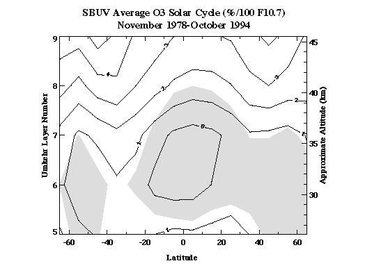
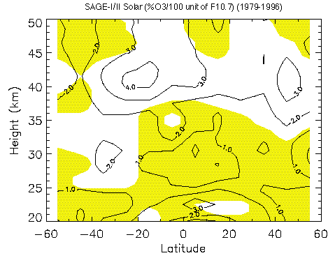
Figure 3.5 Meridional cross sections of the solar signal derived from a) SBUV2 data and b) SAGE I/II data using regression analysis. Contour interval is 1%/100 units of F10.7.
During at least the last three solar cycles, the decadal oscillation has been approximately in phase with proxies for solar ultraviolet flux, and statistical representation is typically based on correlation with the 10.7 cm solar radio flux (F10.7) or the Mg II core-to-wing ratio (Heath and Schlesinger, 1986; DeLand and Cebula, 1993).
The dependence on altitude of the ozone solar cycle signal has been investigated using SBUV/SBUV2 data (Hood et al., 1993; Chandra and McPeters, 1994; McCormack and Hood, 1996) and using SAGE I/II data (Wang et al., 1996). Figure 3.5a,b shows meridional cross sections of the solar signal derived from SBUV/SBUV2 and SAGE I/II data using regression analysis (from the standard model fits discussed above). These plots show percentage ozone changes per 100 units of 10.7 cm solar flux; 130 units is the approximate difference between solar maximum and solar minimum. These data show reasonably consistent patterns in the upper stratosphere, with an in-phase solar cycle variation of 2-4%. Similar sized solar variations in the upper stratosphere are derived from a somewhat longer record (1968-onwards) of Umkehr data (Miller et al., 1995). The SAGE I/II data (with resolution below 25 km) furthermore show a maximum over 23-28 km centred in the tropics (£30oN-S). The vertical integral of these SAGE I/II data results in a column ozone variation of approximately 2%, and this is in reasonable agreement with the TOMS and SBUV/SBUV2 column ozone solar signal derived over the same time period (1979-1996). Note the SBUV/SBUV2 profile data do not extend into the lower stratosphere, and hence this lower stratospheric tropical decadal variation (~ 85% of the column signal) is not resolved (as discussed in Hood, 1997).
Figure 3.6 shows the solar cycle variation derived from the model results of Jackman et al. (1996), who include detailed treatment of the solar spectral characteristics derived from UARS data. This model result shows a broad latitudinal maximum in the upper stratosphere with maximum amplitude near 1.5%; this is similar in altitude dependence but smaller in magnitude (by about 50%) than the satellite results shown in Figure 3.5. The model does not show a maximum in the tropical lower stratosphere (i.e. the maximum seen in SAGE I/II data in Figure 3.5b). Consistent with this, the model column variation is approximately 1%, somewhat less than the 2% derived from the relatively short record of TOMS. Very similar model estimates of the solar cycle variation have been obtained by Brasseur (1993) and Haigh (1994).
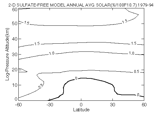
Figure 3.6 Solar cycle variation derived from a 2D photochemical-dynamical model including solar cycle variation of the ultraviolet solar flux responsible for ozone production [Jackman et al. (1996)].
In summary, the decadal variation in upper stratospheric ozone observed in satellite data is similar in spatial pattern to model calculations of the solar cycle, but the observed changes are approximately a factor of two larger than model results. In addition, the satellite data show an in-phase variation in the lower stratosphere not seen in model calculations. Consistent with this, the decadal oscillation in column ozone derived from data is somewhat larger than model predictions. This source of observed-model discrepancy is unresolved at present; it may be due to ozone transport effects that are unresolved in the models, or to uncertainties associated with the relatively short observational record. This uncertain knowledge of solar effects is one limiting factor in understanding long-term ozone variability.
Record low ozone levels observed after the eruption of Mount Pinatubo in 1991 (Gleason et al., 1993) led to a renewed appreciation of the effects of volcanoes on stratospheric ozone. Hofmann and Solomon (1989) proposed such an explanation for relatively small (~2%) ozone losses after El Chichon (in 1982), based on heterogeneous chemistry occurring on the volcanic sulphate aerosols. Observed losses after Pinatubo were substantially larger, of order 5-10% in NH middle-high latitudes (e.g. Gleason et al., 1993; Hofmann et al., 1994; Bojkov et al., 1993; Kerr et al., 1993; Grant et al., 1994; Randel et al., 1995; Coffey, 1996). Numerous modelling studies have shown ozone depletion with similar magnitude and space-time structure (maximising in NH winter 1991-92 and 1992-93) (e.g. Tie et al., 1994; Bekki et al., 1994; Rosenfield et al., 1997). This consistency in modelling the ‘fingerprint’ of Pinatubo on ozone supports confidence in physical understanding of the heterogeneous chemical mechanisms involved.
Recent studies have shown that including realistic time series of sulphate aerosol surface area density in 2-D model calculations of total ozone improves the agreement with observations in the northern hemisphere middle latitudes (Solomon et al., 1996) and in global ozone (Jackman et al., 1996). Thus a primary source of ozone variability appears to be related to the amount of stratospheric sulphate aerosols, which is reasonably well constrained by observations (Thomason et al., 1997). The episodic nature of the volcanic events allows their influence to be isolated, and the effects on trend calculations is minimal unless they occur near one end of the time series (the volcanic time periods are often simply omitted from the trend calculations).
As noted by Solomon et al. (1996), the occurrence of two major volcanic eruptions nine years apart during each of the last two declining phases in solar activity could lead to some confusion in separating volcanic and solar effects on ozone. This will not strongly influence trend estimates for the long time records, but may have implications for isolation of the solar cycle in the short observational record. This is demonstrated using model output in Figure 3.7, where the model results of Jackman et al. (1996) including sulphate aerosol effects are used to calculate the apparent solar cycle variation over 1979-1994; this result should be compared to the 'true' model solar cycle in Figure 3.6 (derived from a 'no-sulphate' model run). This comparison shows a large projection of the aerosol effects in the lower stratosphere onto the solar cycle during this time period; the derived solar signal in the lower stratosphere is a completely spurious result in the aerosol simulation. This result suggests caution should be applied to detailed interpretation of apparent solar cycle variations in the relatively short satellite data record since 1979 (especially for lower stratospheric profile and column ozone).
Attempts to statistically model the volcanic influence on ozone in regression analysis is a relatively novel idea and a topic of current research. One simplified, first-order statistical approach toward separating volcanic and solar effects involves including an explanatory variable linked to the atmospheric aerosol content in multiple regression models (McCormack et al., 1997). This is only an approximate approach since, for example, it neglects the multiplicative effect of increasing chlorine loading during the 1980's (Tie and Brasseur, 1995), or the important effects of temperature variations.
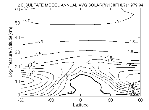
Figure 3.7. Apparent solar cycle variation derived from a 2D photochemical-dynamical model which included solar cycle variation of ultraviolet solar flux and variation of the aerosol concentration due to volcanoes such as El Chichon and Mount Pinatubo [C.H. Jackman, private communication].
Column Ozone
Interannual variability in tropical ozone is dominated by an approximate 2-year cycle, which is closely linked with the quasi-biennial oscillation (QBO) in zonal wind and temperature in the tropical stratosphere. A strong QBO component in ozone is also observed at extra-tropical latitudes in both hemispheres. Analyses of long time records of global satellite data from TOMS have clearly documented characteristics of the global QBO in column ozone (Bowman, 1989; Lait et al., 1989; Chandra and Stolarski, 1991; Randel and Cobb, 1994; Tung and Yang, 1994, Yang and Tung, 1994). The main results of these analyses show: 1) column ozone variations near the equator (£10o latitude), approximately in phase with equatorial zonal winds near 30 hPa, and 2) extra-tropical anomalies over approximately 15o-60o latitude in each hemisphere, approximately out of phase with the tropical signal. The amplitude of the column ozone QBO anomalies is of order 2-4% of the mean ozone amount.
An intriguing and as yet poorly understood aspect of the extra-tropical QBO is that it is seasonally synchronised, such that the QBO influence is observed only during winter-spring of each respective hemisphere. Similar results have been derived from ground-based measurements (e.g. Hamilton, 1989; Yang and Tung, 1994) and other satellite-derived column ozone data (Hasebe, 1983; Hollandsworth et al., 1995).
Besides the QBO signals in the tropics and mid-latitudes, analysis of TOMS data and other long-term records suggest a further region of QBO influence in the winter polar vortices (Oltmans and London, 1982; Garcia and Solomon, 1987; Bowman, 1989; Lait et al., 1989; Randel and Cobb, 1994). The polar ozone QBO is approximately in phase with mid-latitudes (and out of phase with the tropics), and also seasonally synchronised (maximum in spring). Observational evidence for the polar ozone QBO is less statistically significant than that in the tropics or mid-latitudes, at least partly because of the high level of "natural" interannual variability in springtime vortex structure.
Statistical modelling and isolation of the column ozone QBO is straightforward, using a regression analysis tied to the equatorial zonal winds. It is important to include seasonally-dependent coefficients in such regressions to accommodate the seasonally synchronised nature of the mid-latitude QBO. The details of such analyses can depend on the specific altitude of the reference time series (because the QBO propagates downward in time), and some studies include a latitude-dependent time lag. Randel et al. (1995) have used a linear combination of zonal winds over 10-70 hPa as a basis time series for column ozone QBO regressions, and Ziemke et al. (1997) have shown that this provides optimal fits and maximum reduction in variance (and that no time lag is necessary).
Figure 3.8a shows interannual anomalies in TOMS column ozone at the equator, together with this optimal QBO reference time series. The TOMS anomalies at 28° N are shown in Figure 3.8b, together with the QBO fit derived by regression analysis (note the large anomalies during NH winter, approximately out of phase with the tropical QBO variations in Figure 3.8a).
Ozone Profile
The vertical structure of the ozone QBO has been analysed using SAGE II data by Zawodny and McCormick (1991), Hasebe (1994) and by Randel and Wu (1996). Their results show that there is a two-cell vertical structure to the tropical and mid-latitude QBO, peaking in the lower stratosphere (20-27 km) and middle stratosphere (30-38 km), with a node near 28 km. This is shown in Figure 3.9a,b, for anomalies over the equator and at 28° N. The two maxima are approximately in quadrature in the tropics, but are in phase at mid-latitudes. Both the lower and middle stratosphere components contribute important fractions to the column ozone amounts (approximately 2/3 and 1/3 fractions, respectively). The vertical integrals of these SAGE II anomalies are included in the time series shown in Figure 3.8, showing good agreement with the QBO component in the TOMS data.
SAGE II measurements of nitrogen dioxide furthermore show a strong QBO signal in the middle stratosphere (Zawodny and McCormick, 1991; Randel and Wu, 1996), and Chipperfield et al. (1994) demonstrated from modelling results that the two-cell vertical structure in ozone was due to transport (in the lower stratosphere) and reactive-nitrogen associated chemical effects (in the middle stratosphere), respectively.
Accurate statistical modelling of the profile ozone QBO may be accomplished using regression analyses based on two (orthogonal) reference QBO time series (Randel and Wu, 1996), which allows for the continuous vertical propagation observed in the profile anomalies. Alternatively, the fitting can be accomplished by using a single reference time series with variable lag at each latitude and height.

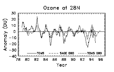
Figure 3.8 Time series of deseasonalized anomalies in TOMS column ozone at the equator and 28°N. Light dashed lines in (a) show the QBO reference time series, derived from an optimal linear combination of zonal winds over 70-10 mb (Randel et al., 1995). Light dashed lines in (b) show the statistical QBO fit at 28°N, derived using seasonally-varying regression. Heavy dashed lines in both panels show column ozone anomalies above 20 km derived from the SAGE II data shown in figure 3.9.
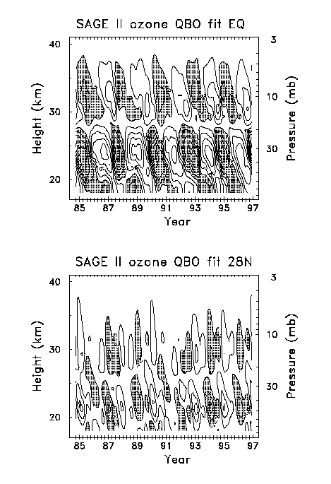
Figure 3.9 Altitude-time sections at the equator (a) and 28°N (b) of SAGE II ozone density anomalies (DU/km) associated with the QBO. Contour values are ± pm 0.2, 0.6, 1.0, ... DU/km with positive values shaded. Note the separate maxima in the lower and middle stratosphere; these contribute about 2/3 and 1/3 of the column amounts, respectively. The vertical integral of these anomalies are included in Figure 3.8.
Ozone is strongly influenced by meteorological variability on both short and inter-annual time scales. Accurate characterisation of such dynamical variations therefore allows increased precision in trend estimates (or at least a reduction in trend uncertainties). An example of "anomalous" meteorological variability is the El Nino-Southern Oscillation (ENSO), which is known to affect column ozone amounts (Shiotani, 1992; Randel and Cobb, 1994). However, the effects of ENSO are mainly longitudinally localised, and the influence on zonal mean ozone is typically less than 1%, so that little reduction in overall variance is gained by including an ENSO proxy in regression models for zonal mean ozone.
With regard to "natural" meteorological variability, Ziemke et al. (1997) have investigated the use of several meteorological fields for use as dynamical proxies for column ozone, including temperature, geopotential height, relative and potential vorticity, and other fields. The strongest correlation (and reduction in regression variance) was obtained using lower stratospheric temperature data (from Microwave Sounding Unit (MSU) Channel 4). An important point to note is that lower stratospheric temperatures also exhibit negative trends (Miller et al., 1992; Spencer and Christy, 1993), with spatial structure similar to that of observed ozone trends (Randel and Cobb, 1994). Modelling studies suggest that much of the observed temperature trend can be explained as a radiative response to the observed ozone changes (Ramaswamy et al., 1996). In addition, a portion of this temperature trend may be of dynamical origin (Hood et al., 1997). In either case, using the full time series of temperature data (including a long-term trend) as a dynamical proxy can result in a change (underestimate) in the derived ozone trends. A practical alternative is to de-trend the temperature data prior to use in the regression model, and use the de-trended data to model the high-frequency components of the ozone variance. The overall effect of including such a dynamical proxy is a small reduction in the derived trend uncertainty estimates for total ozone (Ziemke et al., 1997).
Summary
Decadal variations are a ubiquitous feature of ozone observations, in addition to QBO and faster time scale dynamical variability. These latter terms have little influence on calculation or interpretation of trends. Much of the observed decadal changes are approximately in phase with the solar cycle for the observational record, suggesting a solar mechanism. However, current model calculations of the solar effect show some inconsistencies with observations (in terms of magnitude and lower stratospheric response), and this limits confidence in our detailed understanding. There is also likely a confusion of solar and volcanic signals for the recent record. Although these effects have relatively small impacts on trend estimates, it does limit our ability to interpret decadal variability.
![]()