Previous: Introduction Next: Conclusions Up: Ext. Abst.

Results

Results are presented for 15 year ensemble means from two simulations respectively for typical conditions of 1990 ("present" simulation) and of 1960 ("near past" simulation). The AMIP average sea surface temperature, SST, have been used for the "present" simulation and GISS-HADLEY (average 1951-1960) for the "near past" simulation. See also Brühl et al. poster in Session 1. Results are also presented from a 15 year simulation (hereafter FKO3) with the GCM component only, with specified observed ozone climatology (Fortuin and Kelder, 1998), present conditions for greenhouse gases and the AMIP SST. For a detailed evaluation of the simulations with respect to observations see Brühl et al. poster in Session 1.

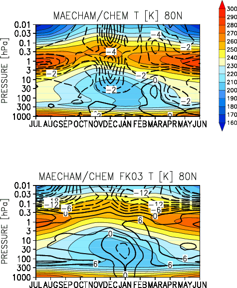
Figure 1: (upper) In color, ensemble monthly zonal mean temperature [K] from the "near past" simulation. Time - pressure section at 80N. Black contour: Difference, "present" -"near past" simulations, of the ensemble monthly zonal mean temperature [Contour: 1 K]. Time - pressure section at 80N. (lower) In color, ensemble monthly zonal mean temperature [K] from the FKO3 simulation with the GCM component only, with specified observed ozone climatology (Fortuin and Kelder, 1998) and present conditions for greenhouse gases. Time - pressure section at 80N. Black contour: Difference, "present" - FKO3 simulations, of the ensemble monthly zonal mean temperature [Contour: 3 K]. Time - pressure section at 80N.

Figure 1 (upper) shows the seasonal evolution of the warm stratopause, higher in winter, the cold summer mesopause, and the cold (~210 K) polar lower stratosphere in winter. There is general cooling of the atmosphere: Cooling of the stratopause, largest in summer (~6 K) and complicated cooling pattern from October to March, presumably affected by dynamical variability. Weak warming mainly confined to the troposphere.

Figure 1 (lower) shows a warming (up to 9 K in summer) in the lowermost stratosphere (~200 hPa), due to downward and poleward transport of ozone in the "present" simulation with interactive chemistry. During the polar night the "present" simulation is colder. The large cooling in the mesosphere (largest at the summer pole) is due to diurnal cycle variations in ozone (minimum in sunlight) included in the interactive simulation. The FKO3 ozone is instead a monthly mean, extrapolated from the middle to the upper mesosphere.

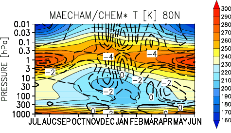
Figure 2: As in Figure 1 (upper), but the ensemble mean of the "present" simulation is based on 13 years only, to exclude the winter season when a particularly strong (but not major) stratospheric warming occurred in November. Note a more gradual cooling of the middle stratosphere in early winter. The December cooling is decreased (wrt Figure 1) in the upper stratosphere. The March weak warming is persistent. The alternate modulation of the temperature difference suggests a change in the seasonal stability of the polar vortex: more active in early winter, quiescent in mid winter and again more active in spring, in the "present" with respect to "near past" simulation.

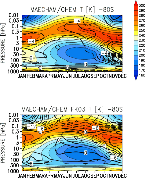
Figure 3: As Figure 1, but at 80S, and 2 K black contour in upper panel. Note the pronounced descent of the warm stratopause in late winter and the quite cold (~180 K) polar lower stratosphere in winter. As for the northern hemisphere, there is general cooling of the atmosphere, i.e., around the stratopause and in the lower stratosphere from September to December-January. The latter (16 K of difference in November) is associated with ozone destruction by heterogeneous chemistry. The warming above is the dynamical response: increased descending motions in the polar region. See Figure 4. As for the northern hemisphere, with interactive chemistry the mesosphere cools, especially in summer, and the lowermost stratosphere (~200 hPa) warms. The cooling in November (due to the ozone hole) is consistent with the fact that the FKO3 ozone climatology is more representative of the 1980s, while the "present" simulation of the 1990s.

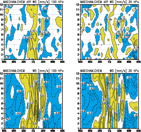
Figure 4: (upper) Difference, "present" - "near past", of the ensemble monthly mean residual vertical velocity [mm/s]. Latitude - time section (left) at 100 hPa and (right) at 30 hPa. Contour: 0.1 mm/s. Yellow is above 0.05 mm/s, blue below -0.05 mm/s. Month 1 is January. (lower) Ensemble monthly mean residual vertical velocity [mm/s] from the "near past" simulation. Latitude - time section (left) at 100 hPa and (right) at 30 hPa. Contour: 0.1 mm/s.Yellow is above 0.05 mm/s, blue below -0.05 mm/s. Month 1 is January

At 100 hPa, Figure 4 (upper) shows increased equatorial upwelling relatively homogeneous in time, associated with cooling, and consistent with a localized decrease in ozone. Given the large vertical gradient in ozone, finer vertical resolution would help in characterizing the tropopausal changes. Compensating downwelling larger in the subtropics.

At 30 hPa, Figure 4 (upper) shows that at northern polar latitudes, the donwelling from December to March is increased, indicating larger dynamical activity in the "present" simulation, in spite of the polar average cooling (Figure 1). South Pole December: Increased dowelling consistent with the persistence of the polar vortex (Figure 3).

At 100 hPa, Figure 4 (lower): Upwelling in the tropics and downwelling in the extratropics. Note the seasonal shift of the latitude where the residual vertical velocity change sign. The magnitude of the tropical upwelling (~0.5 mm/s) is consistent with estimate of it from comparison of the simulated water vapor with HALOE observations.

At 30 hPa, Figure 4 (lower): Downward velocities in the extratropics, their magnitude larger in mid winter. Rich latitudinal structure in tropical upwelling.