Previous: Model Description Next: Concluding Remarks Up: Ext. Abst.
Results
1. Temperature in the nudging CTM
CCSR/NIES GCM has so-called cooling bias in temperature in the lower stratosphere and upper troposphere as most GCMs in the world have. The nudging CTM prevented such cooling biases and greatly improved the temperature and wind fields. However, there is still discrepancy in these fields between the nudging CTM and observation. The zonal-mean temperature difference between the ECMWF data and the CTM was less than 2 K in the CTM with the nudging time scale of 1 day. The maximum difference occurred in the lower stratosphere in the winter Pole. The difference in the upper troposphere over the tropics was about 1.5 K. Such cooling bias in this region affects the water vapor amount in the model stratosphere. Thus, the water vapor amount in the stratosphere of the nudging CTM is insufficient. The temperature and wind field difference depends on the nudging time scale. In general, a shorter nudging time scale makes the smaller difference. However, the shorter time scale tends to make noise in the model. For example, if the time scale is shortened to 0.1 day, a noisy pattern appears in H2O distribution in the stratosphere, and the flux from the troposphere through the tropopause was erroneously increased and the calculation failed. The shorter time scales also prevent the buildup of a high concentration of ClO over the Antarctica in September and October. On the other hand, with a longer time scale, the differences in temperature and wind fields become larger. For example, with a time scale of 5 days, the cooling bias of the nudging CTM is about 2 K in the tropical upper troposphere and more than 5 K in the polar stratosphere.
2. Photolysis rates
Photolysis rates of chemical species were calculated directly from the radiation flux convergence in each atmospheric layer of the model and the Schumann-Runge parameterizations. To verify the calculation, the calculated photolysis rate profiles at local noon on March 22 were compared with those of the JPL-97 profiles. The calculated profiles were quite close to those of JPL-97, and the result shows that the calculations were successful in the model.
3. Total ozone
3.1 Dependence of horizontal resolution
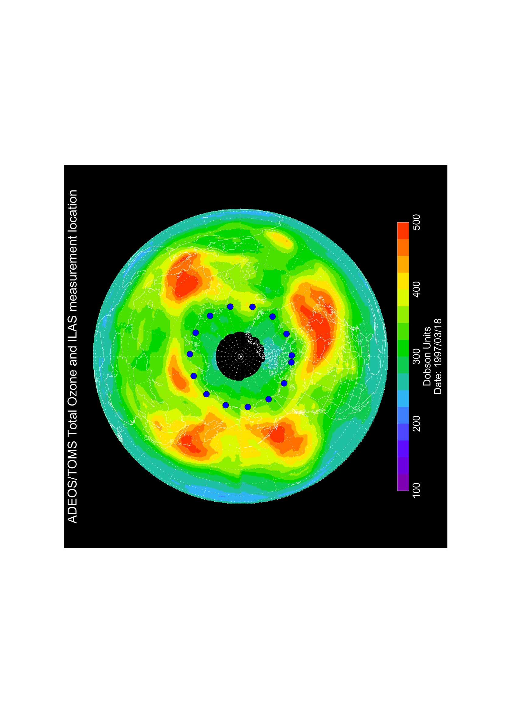
Figures 1, 2, and 3 show the total ozone distribution in the Arctic region observed by TOMS on March 18, 1997, and those calculated by the T21(5.6 5.6) model and the T42(2.8 2.8) model at 0:00 UT on the same day, respectively. These distributions were calculated with the nudging time scale of 1 day. The distribution is simulated well, although the total ozone amount in the high latitudes is a little higher than the observation. The distribution was also calculated by T10 (11.2 11.2) model, but the low resolution model was not capable to simulate the Arctic ozone distribution accurately. The improvement of the Arctic ozone distribution from the T21 model to the T42 model was not substantial for the planetary scale distribution simulation. But the use of the T42 model may be necessary for comparisons of the vertical distribution and the time variation with the observations at a fixed location, because the observation values at the fixed point are considerably affected by the small scale distributions. It was found that at least horizontal T21 resolution is necessary for realistic simulations of Arctic ozone distribution.
Figure 1. Total ozone distribution in the Arctic observed by ADEOS/TOMS on 18 March 1997.
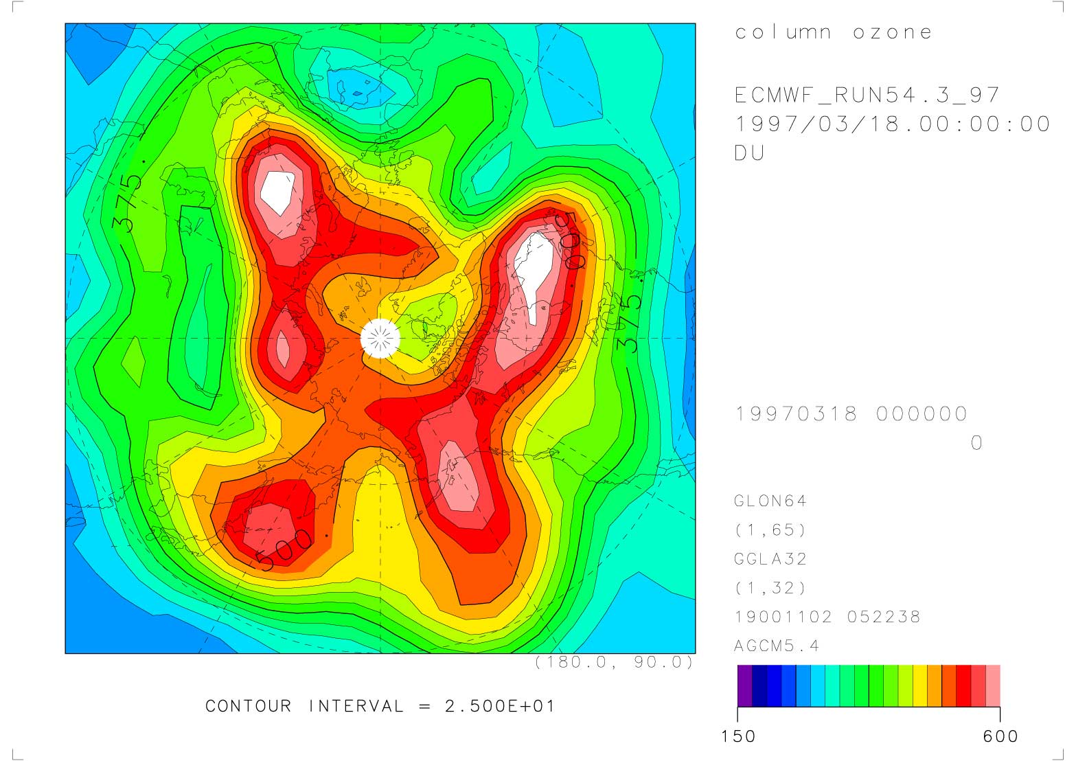
Figure 2. Total ozone distribution in the Arctic at 0:00 UT on 18 March 1997 calculated by the T21 CCSR/NIES nudging CTM. The nudging time scale is 1 day.
Figure 3. Same as Figure 2, but calculated by the T42 model.
3.2 Dependence of nudging time scale
Figure 4 shows the Arctic ozone distribution at 0:00 UT on March 18, 1997 calculated by the T21 model, but with the nudging time scale of 5 days. The pattern of the total ozone distribution is slightly trailing in the zonal direction.
Figure 4. Same as Figure 2, but calculated with the nudging time scale of 5 days.
3.3 Comparison of the distribution between with and without heterogeneous chemistry
Figure 5 shows the Arctic ozone distribution on March 18, 1997 calculated by the T21 model, but without heterogeneous chemistry. The total ozone difference was between 30 DU and 70 DU in the north of 70 N, compared with Figure 4.
Figure 5. Same as Figure 4, but without heterogeneous chemistry.
4. Vertical profiles-comparison with ILAS observation
The vertical distribution of O3 N2O, and HNO3 mixing ratio of the T42 model with the nudging time scale of 1 day was compared in Figures 6, 7, and 8 with ILAS V05.00 data, which were analyzed by ILAS science team. The data point is near Kiruna, inside the Arctic polar vortex near the vortex boundary.
Figure 6. Comparison between O3 profiles of nudging CTM at 68.368N, 30.938E at 0:00 UT on 18 March 1997 (dotted line), and of ILAS V05.10 O3 at 69.38N, 30.63E at 15:54 on 17 March 1997 (solid line).
Figure 7. Same as Figure 6, but comparison of N2O profiles.
Figure 8. Same as Figure 6, but comparison of HNO3 profiles.
5. Zonal mean meridional distributions of reactive nitrogen, reactive chlorine, and reactive bromine
Maximum zonal-mean volume mixing ratio of NOy in the model was about 16 ppmv around 40 km over the tropics and about 15 ppmv around 30 km over mid and high latitudes. The maximum zonal-mean volume mixing ratios of Cly and Bry in the upper stratosphere was 3.5 ppbv and 21 pptv. These computed values are quite reasonable for mid-90s.
6. Vertical distributions of CFCs
Figure 9 shows the calculated CFC profiles at 68.37N, 19.69E on 19 March 1997. The profiles of CFC-11, CFC-12, CFC-113, and halon-1211 were compared with those measured at Kiruna on March 18 by Shirai et al. (2000). The vertical distributions of these gases that has the source at the surface were also simulated well.
Figure 9. CFC profiles of the nudging CTM at 68.37N, 19.69E at 0:00 UT on 19 March 1997.
Figure 10. Same as Figure 7, but the CTM profile without photolysis at the spectra less than 200 nm (dotted line).
Figure 11. Same as Figure 9, but the CTM profiles without photolysis at the spectra less than 200 nm.
7. Effcts of Schumann-Runge bands
In the previous version of the nudging CTM, photolysis processes of N2O and CFCs at the spectra less than 200 nm were not included. Then, there were some problems in the calculated vertical profiles of these species. The altitudes where the concentrations of those species decrease rapidly from the tropospheric values to much lower stratospheric values due to photolysis were a few kilometer higher than the observations. The profiles were greatly improved by introducing Minschwaner et al.(1993)¡Çs radiation flux parameterization in the Schumann-Runge bands between 177.5 nm and 200.0 nm.