1National Institute for Environmental Studies, Tsukuba, Ibaraki
305-0053, Japan
2Center for Climate System Research, University of Tokyo, 4-6-1
Komaba, Meguro-ku, Tokyo, 153-8904, Japan
3Fujitsu FIP, 2-45 Aomi, Koutou-ku, Tokyo 135-8686, Japan
FIGURES
Abstract
Development of a new chemical transport model is described. The model has been developed based on CCSR/NIES AGCM. A nudging technique is used to assimilate the temperature and horizontal wind velocity data into the calculation values of the GCM. Photolysis rates of chemical species are directly calculated in the model by the two-stream approximation of the radiation transfer that is used for atmospheric heating rate calculations. Column amount distribution of ozone and the seasonal variation, and the distributions of HOX, NOX, ClOX, and BrOX in 1997 are simulated by the model with T10, T21, and T42 horizontal resolutions. It is shown that the T21 and T42 models simulate the global distributions of chemical species realistically, although the total ozone amount in the high latitudes is somewhat larger than the observation. The results are also compared between the nudging time scales of 1 day and 5 days, and between with and without heterogeneous chemistry
Introduction
Chemical transport model is a powerful tool for studying the mechanisms of 3-D distributions of chemical species in the atmosphere. Several three-dimensional chemical transport models have been developed, and the developments are being continued for better understanding of global distributions and variations of many kinds of chemical constituents as well as the ozone depletion in the Antarctic and in the Arctic (e.g. Brassuer et al., 1997; Lefevre et al., 1998; Chipperfield, 1999). In order to develop a fully coupled, chemical-radiative-dynamical interactive model for prediction of future ozone layer, chemistry-radiation-coupled scheme must be incorporated into a GCM. The final goal of our study is to develop a 3-D chemical model that can be used both as a Chemical Transport Model constrained by meteorological data, and as a chemical-radiative-dynamical fully interactive GCM. Such model will enable us to check the chemical scheme and the advection scheme of the model by comparisons with observations. At the same time, a reliable prediction of future ozone in the chemical-radiative-dynamical interactive model will be possible. In this paper, development of a new CTM is described, then the calculated distributions and variations of several chemical species in 1997, when ILAS O3, N2O, and HNO3 data were available, are shown and compared with the observations.
Model Description
A stratospheric nudging Chemical Transport Model has been developed in NIES based on CCSR/NIES AGCM (Center for Climate System Research, University of Tokyo/National Institute for Environmental Studies Atmospheric General Circulation Model), which has been developed by Numaguti (1993), Numaguti et al. (1995), and Numaguti et al. (1997). A detailed description of the dynamical, radiative, and chemical component of a privious version of our chemistry coupled GCM was given in Takigawa et al. (1999). The model has 30 atmospheric layers, as shown in Table 1 of Takigawa et al. (1999). The top level is located around 70 km. The new nudging CTM was developed by incorporating a nudging module into the model and by replacing the chemical scheme with a more sophisticated one that has been developed in NIES and used in a 1-D coupled chemistry-radiation model (Akiyoshi, 2000).
The new model includes BrOX chemistry and heterogeneous reactions on NAT/ICE clouds in the stratosphere as well as the OX, HOX, NOX, hydrocarbons, and ClOX gas phase chemical reactions for the stratosphere. The chemical species and the families predicted numerically in this model are OX (O(1D) + O + O3), NOX (N + NO + NO2 + NO3), ClOX (Cl + ClO + 2Cl2O2 + ClOO + OClO), BrOX (Br + BrO), CH4, CO, N2O, CCl4, CFCl3, CF2Cl2, CH3CCl3, CH3Cl, CClF2CCl2F, CHClF2, H2O, HF, H2O2, HNO3, HNO4, N2O5, ClONO2, HCl, HOCl, CF2ClBr, CF3Br, CF2Br2, CHBr3, CH3Br, HBr, HOBr, BrONO2, Cl2, Br2, NOy (NOX + HNO3 + HNO4 + 2N2O5 + ClONO2 + BrONO2), Cly (ClOX + HCl + HOCl + ClONO2 + BrCl + 2Cl2), and Bry (BrOX + HBr + HOBr + BrONO2 + BrCl + 2Br2). CH3O2, CH3OOH, CH2O, OClO, and BrCl were also predicted, but photochemical equilibrium concentrations were assumed during daytime. HNO4 was also predicted, but photochemical equilibrium concentrations were assumed in the troposphere during daytime. The HOX family (H + OH + HO2) and following species are assumed to be in photochemical equilibrium; O(1D), O, O3, H, OH, HO2, HOX, N, NO, NO2, NO3, CH3, CHO, Cl, ClO, Cl2O2. ClOO, Br, and BrO. The concentrations of these species were calculated by partition equations in the families. Nighttime consentrations of O(1D), O, H, OH, N, NO, CH3, CH3O, CHO, Cl, and ClOO were assumed to be zero.
Thirteen heterogeneous reactions were considered in the model. These reactions were tabulated in Table 2 of Sessler et al. (1996). The code for a box model version of the SLIMCAT model was incorporated into the nudging CTM. In this work, only NAT and ICE were considered as PSCs.
Photolysis rates of chemical species were calculated directly from the outputs of the solar radiation fluxes in the model. The solar energy absorbed by all radiatively active chemical species, which was calculated by the convergence of solar radiation fluxes in an atmospheric layer, was distributed into the energy absorbed by each chemical species, weighted by absorption cross sections of chemical species (Akiyoshi, 2000).
The photolysis processes in the Schumann-Runge bands of H2O2, N2O, NO2, HNO3, HNO4, N2O5, ClONO2, HCl, HOCl, Cl2O2, CCl4, CFCl3, CF2Cl2, CH3CCl3, CH3Cl, CClF2CCl2F, BrONO2, BrCl, HBr, CF2ClBr, CF3Br, CF2Br2, CH3Br, CHBr3 were not included in the previous versions of our chemical 3-D models. The CCSR/NIES AGCMs, which are the basic frame of the nudging CTM, do not include the ultraviolet radiation less than 200 nm. Thus in the new CTM, the photolysis rates in the Schumann-Runge bands were calculated separately by using the Schumann-Runge band radiation flux parameterization developed by Minschwaner et al. (1993), and added to the photolysis rates at wavelengths more than 200 nm that were computed by the radiation code of the CCSR/NIES AGCM itself. The Schumann-Runge photolysis of NO was calculated by using Allen and Frederick (1982)'s parameterization.
The zonal wind velocity, the meridional wind velocity, and the temperature of ECMWF data were input at 0:00 UT every day, interpolated linearly with respect to the time step of the model, which is variable between 20 minutes and several minutes according to computation stability. Then the interpolated values were assimilated into the model with the nudging method,
dx/dt = - (x-xobs)/?Ó, x = u, v, T,
where u is zonal wind velocity, v is meridional wind velocity, and T is temperature, x is GCM values of u, v, and T, xobs is the ECMWF data values (observation values), ?Óis the time scale of nudging. The time scales of 1 day and 5 days were used for this study. Above 10 hPa, where no ECMWF data exist, monthly, zonal-mean CIRA temperature data were input into the model every month, and interpolated linearly with respect to the model time step, and nudged to the zonal-mean values of the model temperature. Thus vertical wind velocity was calculated in the model by the continuity equation.
Results
1. Temperature in the nudging CTM
CCSR/NIES GCM has so-called cooling bias in temperature in the lower stratosphere and upper troposphere as most GCMs in the world have. The nudging CTM prevented such cooling biases and greatly improved the temperature and wind fields. However, there is still discrepancy in these fields between the nudging CTM and observation. The zonal-mean temperature difference between the ECMWF data and the CTM was less than 2 K in the CTM with the nudging time scale of 1 day. The maximum difference occurred in the lower stratosphere in the winter Pole. The difference in the upper troposphere over the tropics was about 1.5 K. Such cooling bias in this region affects the water vapor amount in the model stratosphere. Thus, the water vapor amount in the stratosphere of the nudging CTM is insufficient. The temperature and wind field difference depends on the nudging time scale. In general, a shorter nudging time scale makes the smaller difference. However, the shorter time scale tends to make noise in the model. For example, if the time scale is shortened to 0.1 day, a noisy pattern appears in H2O distribution in the stratosphere, and the flux from the troposphere through the tropopause was erroneously increased and the calculation failed. The shorter time scales also prevent the buildup of a high concentration of ClO over the Antarctica in September and October. On the other hand, with a longer time scale, the differences in temperature and wind fields become larger. For example, with a time scale of 5 days, the cooling bias of the nudging CTM is about 2 K in the tropical upper troposphere and more than 5 K in the polar stratosphere.
2. Photolysis rates
Photolysis rates of chemical species were calculated directly from the radiation flux convergence in each atmospheric layer of the model and the Schumann-Runge parameterizations. To verify the calculation, the calculated photolysis rate profiles at local noon on March 22 were compared with those of the JPL-97 profiles. The calculated profiles were quite close to those of JPL-97, and the result shows that the calculations were successful in the model.
3. Total ozone
3.1 Dependence of horizontal resolution
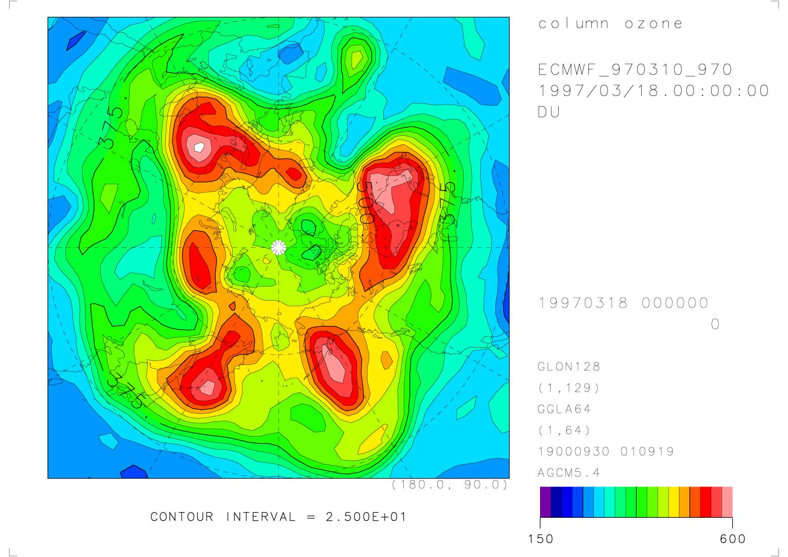
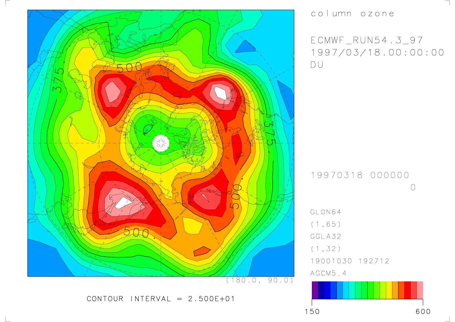
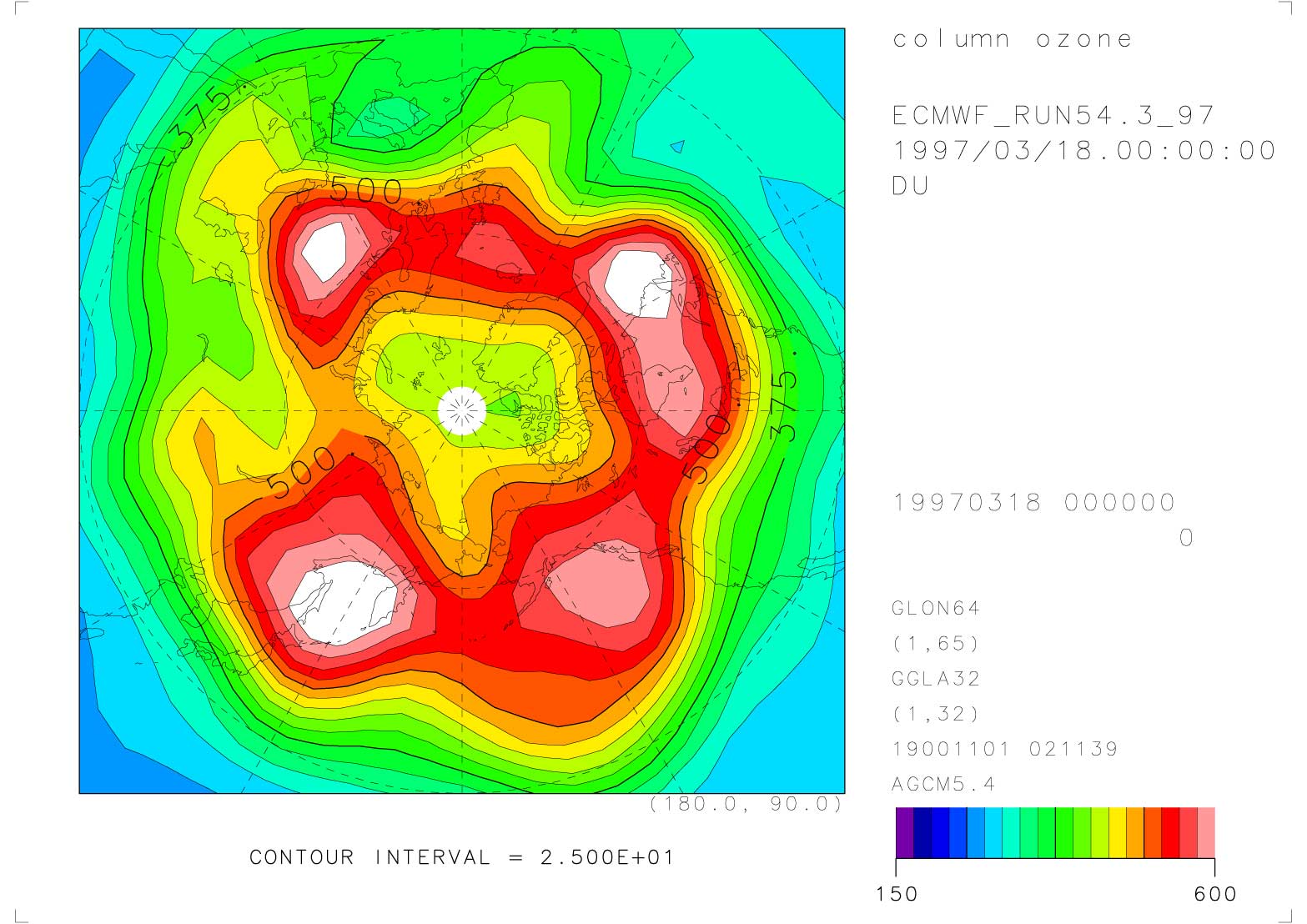
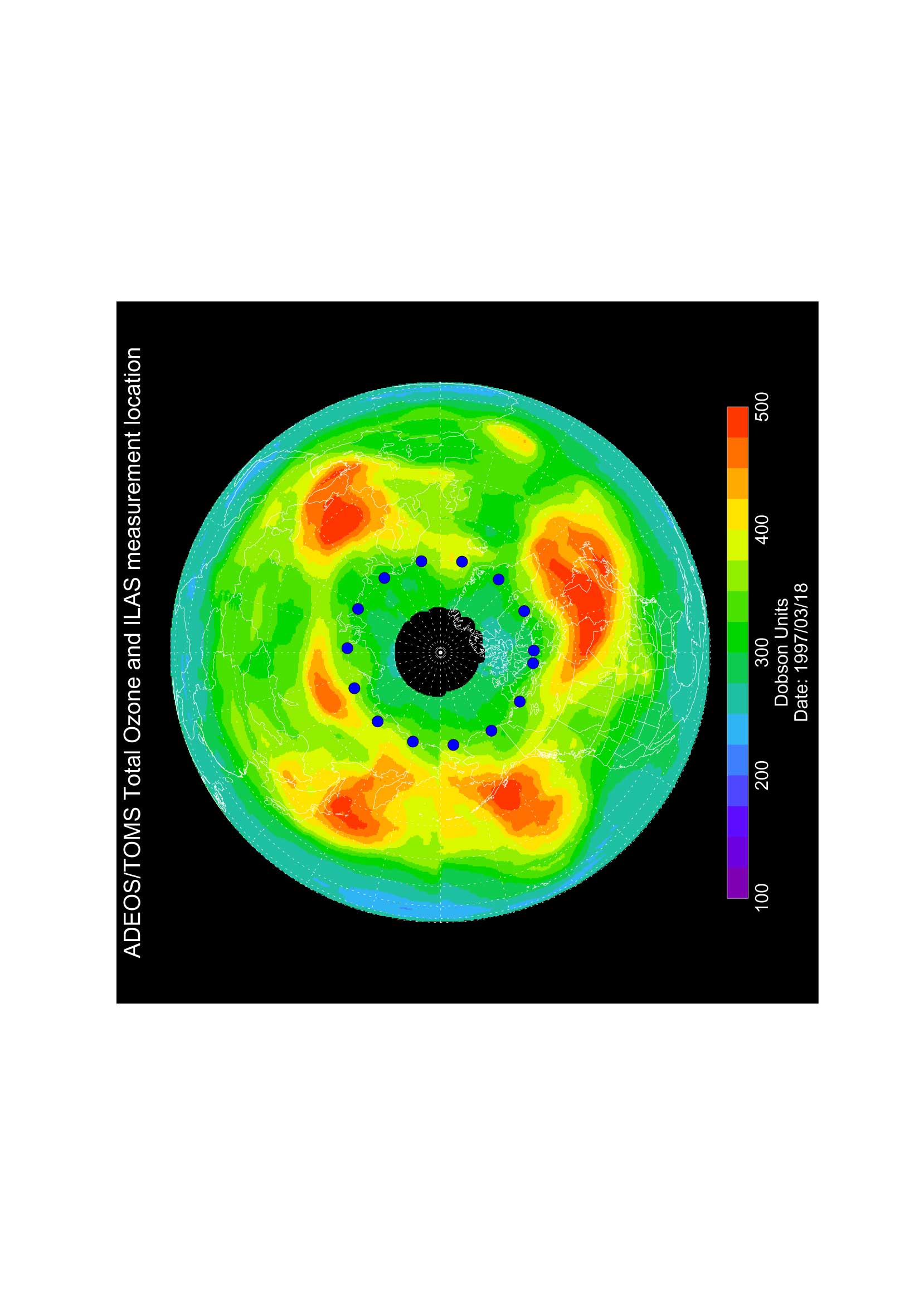
Figures 1, 2, and 3 show the total ozone distribution in the Arctic region observed by TOMS on March 18, 1997, and those calculated by the T21(5.6 5.6) model and the T42(2.8 2.8) model at 0:00 UT on the same day, respectively. These distributions were calculated with the nudging time scale of 1 day. The distribution is simulated well, although the total ozone amount in the high latitudes is a little higher than the observation. The distribution was also calculated by T10 (11.2 11.2) model, but the low resolution model was not capable to simulate the Arctic ozone distribution accurately. The improvement of the Arctic ozone distribution from the T21 model to the T42 model was not substantial for the planetary scale distribution simulation. But the use of the T42 model may be necessary for comparisons of the vertical distribution and the time variation with the observations at a fixed location, because the observation values at the fixed point are considerably affected by the small scale distributions. It was found that at least horizontal T21 resolution is necessary for realistic simulations of Arctic ozone distribution.
Figure 1. Total ozone distribution in the Arctic observed by ADEOS/TOMS on 18 March 1997.
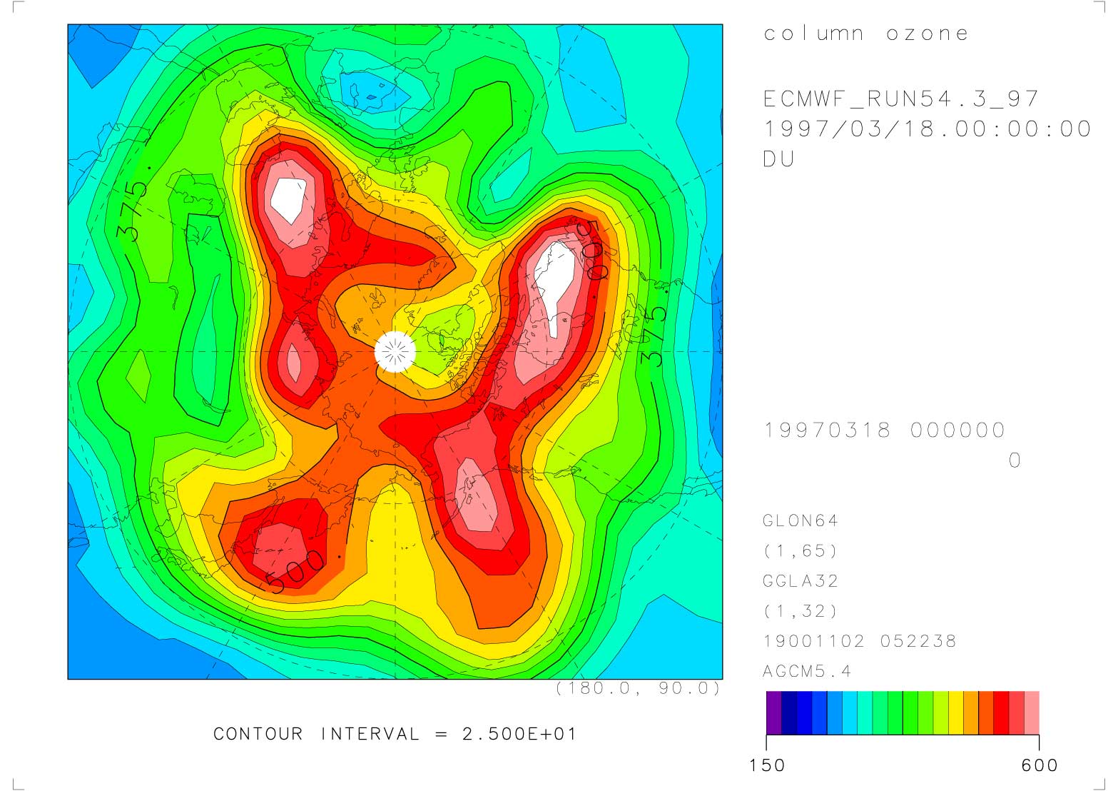
Figure 2. Total ozone distribution in the Arctic at 0:00 UT on 18 March 1997 calculated by the T21 CCSR/NIES nudging CTM. The nudging time scale is 1 day.
Figure 3. Same as Figure 2, but calculated by the T42 model.
3.2 Dependence of nudging time scale
Figure 4 shows the Arctic ozone distribution at 0:00 UT on March 18, 1997 calculated by the T21 model, but with the nudging time scale of 5 days. The pattern of the total ozone distribution is slightly trailing in the zonal direction.
Figure 4. Same as Figure 2, but calculated with the nudging time scale of 5 days.
3.3 Comparison of the distribution between with and without heterogeneous chemistry
Figure 5 shows the Arctic ozone distribution on March 18, 1997 calculated by the T21 model, but without heterogeneous chemistry. The total ozone difference was between 30 DU and 70 DU in the north of 70 N, compared with Figure 4.
Figure 5. Same as Figure 4, but without heterogeneous chemistry.
4. Vertical profiles-comparison with ILAS observation
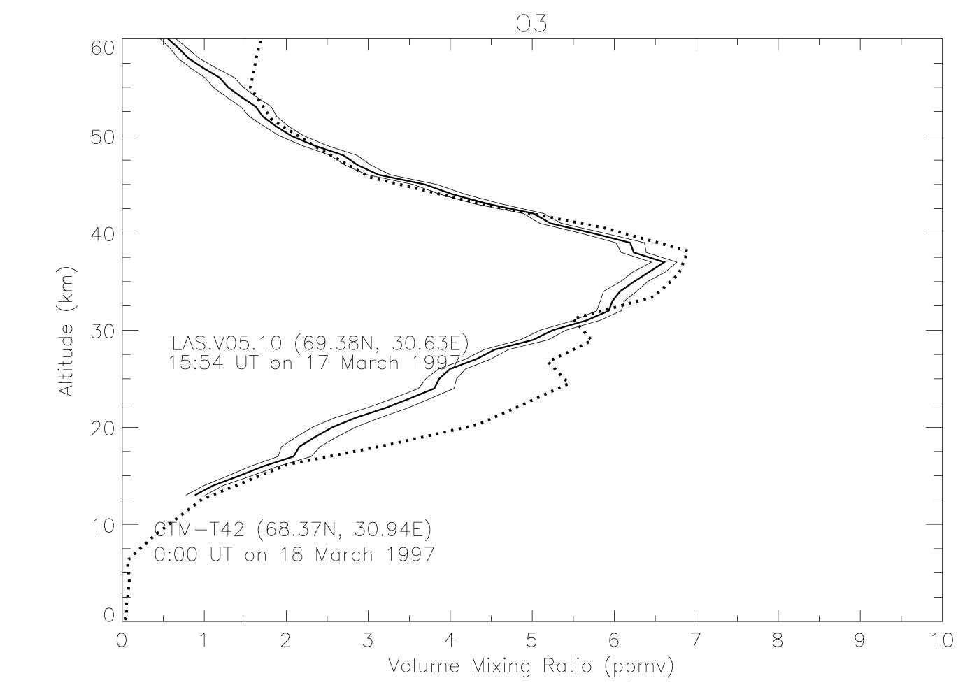
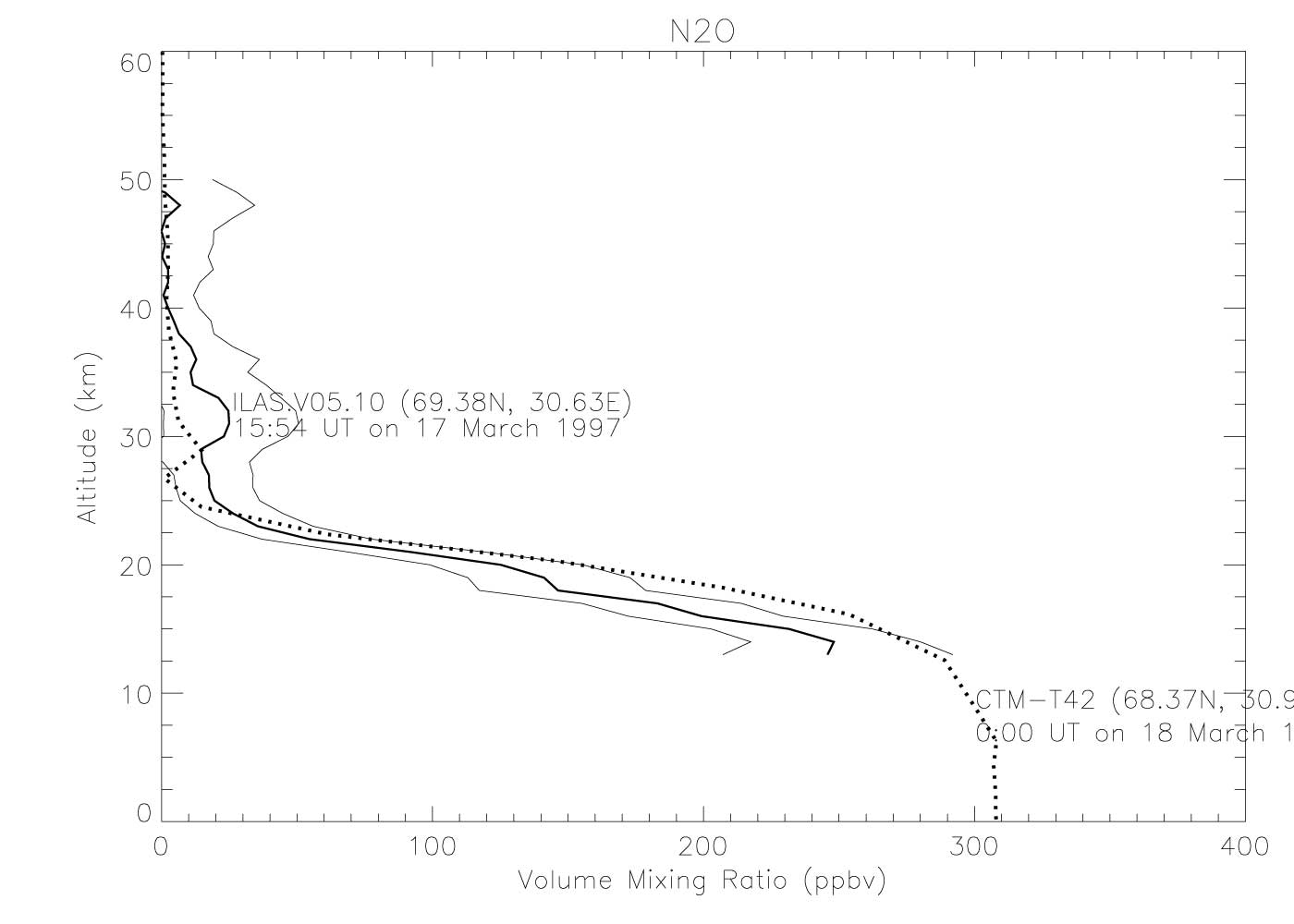
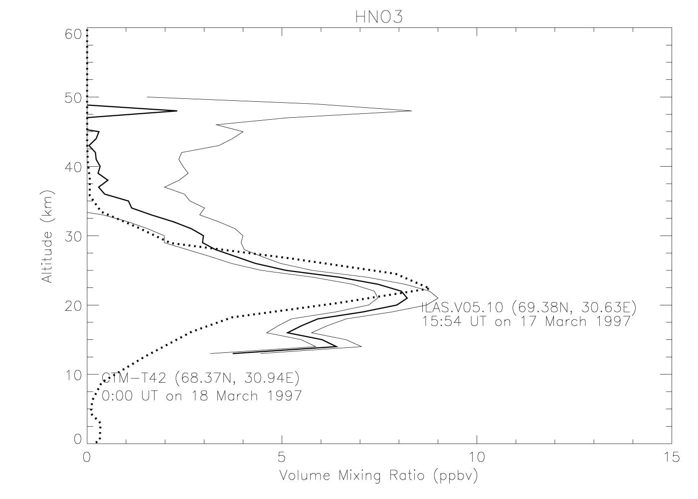
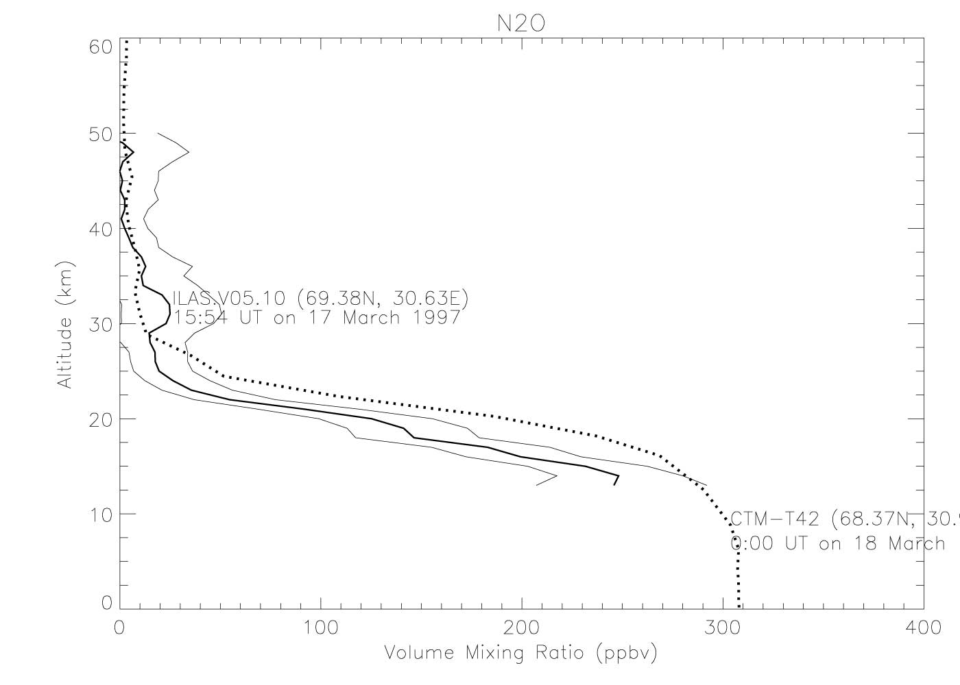
The vertical distribution of O3 N2O, and HNO3 mixing ratio of the T42 model with the nudging time scale of 1 day was compared in Figures 6, 7, and 8 with ILAS V05.00 data, which were analyzed by ILAS science team. The data point is near Kiruna, inside the Arctic polar vortex near the vortex boundary.
Figure 6. Comparison between O3 profiles of nudging CTM at 68.368N, 30.938E at 0:00 UT on 18 March 1997 (dotted line), and of ILAS V05.10 O3 at 69.38N, 30.63E at 15:54 on 17 March 1997 (solid line).
Figure 7. Same as Figure 6, but comparison of N2O profiles.
Figure 8. Same as Figure 6, but comparison of HNO3 profiles.
5. Zonal mean meridional distributions of reactive nitrogen, reactive chlorine, and reactive bromine
Maximum zonal-mean volume mixing ratio of NOy in the model was about 16 ppmv around 40 km over the tropics and about 15 ppmv around 30 km over mid and high latitudes. The maximum zonal-mean volume mixing ratios of Cly and Bry in the upper stratosphere was 3.5 ppbv and 21 pptv. These computed values are quite reasonable for mid-90s.
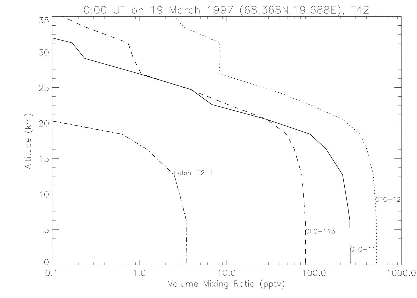
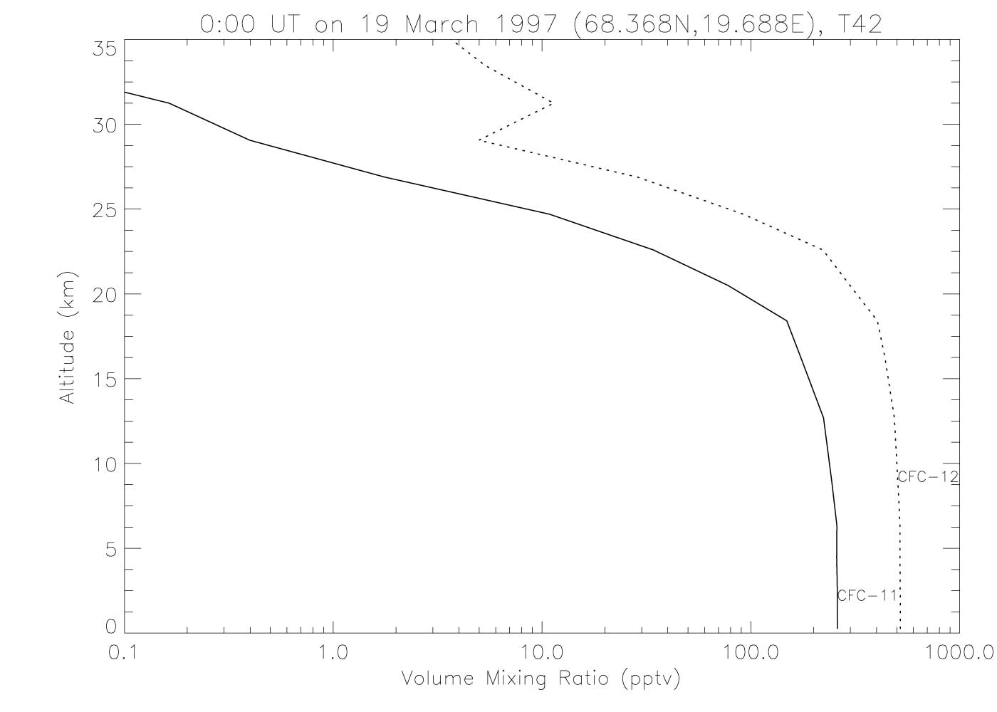
6. Vertical distributions of CFCs
Figure 9 shows the calculated CFC profiles at 68.37N, 19.69E on 19 March 1997. The profiles of CFC-11, CFC-12, CFC-113, and halon-1211 were compared with those measured at Kiruna on March 18 by Shirai et al. (2000). The vertical distributions of these gases that has the source at the surface were also simulated well.
Figure 9. CFC profiles of the nudging CTM at 68.37N, 19.69E at 0:00 UT on 19 March 1997.
Figure 10. Same as Figure 7, but the CTM profile without photolysis at the spectra less than 200 nm (dotted line).
Figure 11. Same as Figure 9, but the CTM profiles without photolysis at the spectra less than 200 nm.
7. Effcts of Schumann-Runge bands
In the previous version of the nudging CTM, photolysis processes of N2O and CFCs at the spectra less than 200 nm were not included. Then, there were some problems in the calculated vertical profiles of these species. The altitudes where the concentrations of those species decrease rapidly from the tropospheric values to much lower stratospheric values due to photolysis were a few kilometer higher than the observations. The profiles were greatly improved by introducing Minschwaner et al.(1993)¡Çs radiation flux parameterization in the Schumann-Runge bands between 177.5 nm and 200.0 nm.
Concluding Remarks
The nudging Chemical Transport Model simulated 3-D distributions and seasonal variations of chemical species, although there is still small discrepancy between the calculations results and the observations in temperature, wind field, absolute amount of total ozone in the Arctic region. The calculations with the STS/ICE scheme are also going on, and the results and comparison with observations will be shown in the near future. Since it is easy to modify the model into a full-coupled chemistry GCM, the model will be used both as a CTM and as a chemical-radiative-dynamical full interactive GCM for atmospheric chemistry-transport studies and for prediction of the future ozone layer.
Acknowledgments.
Computations were made on the NEC SX-4 in NIES. The GFD-DENNOU library 5.0.1 and the GTOOL 3.5 was used for Figures 2, 3, 4, and 5.
References
Akiyoshi, H., Modeling of chemistry and chemistry-radiation coupling processes for the middle atmosphere and a numerical experiment on CO2 doubling with a 1-D coupled model, J. Meteor. Soc. Japan, 78, 563-584, 2000.
Allen, M., and J. E. Frederick, Effective photodissociation cross sections for molecular oxygen and nitric oxide in the Schumann-Runge bands, J. Atmos. Sci., 39, 2066-2075, 1982.
Brasseur, G. P., X. Tie, P. J. Rasch, and F. Lefevre, A three dimensional simulation of the Antarctic ozone hole: Impact of anthropogenic chlorine on the lower stratosphere and upper troposphere, J. Geophys. Res., 102, 8909-8930, 1997.
Chipperfield, M. P., Multiannual simulations with a three-dimensional chemical transport model, J. Geophys. Res., 104, 1781-1805, 1999.
Lefevre, F., F. Figarol, K. S. Carslaw, and T. Peter, The 1997 Arctic ozone depletion quantified from three-dimentional model simulations, Geopyhs. Res. Lett., 25, 2425-2428, 1998.
Minschwaner, K., R. J. Salawitch, and M. B. McElroy, Absorption of solar radiation by O2: Implications for O2 and lifetimes of N2O, CFCl3, and CF2Cl2, J. Geophys. Res., 98, 10543-10561, 1993.
Numaguti, A., Dynamics and energy balance of the Hadley circulation and the tropical precitipation zones: Significance of the distribution of evaporation, J. Atmos. Sci., 50, 1874-1887, 1993.
Numaguti, A., M. Takahashi, T. Nagajima, and A. Sumi, Development of an atmospheric general circulation model. in Reports of a New Program for Center Basic Research Studies, Studies of Global Environment Change With Special Reference to Asia and Pacific Regions, Rep. I-3, pp.1-27, CCSR. Tokyo, 1995.
Numaguti, A., S. Sugata, M. Takahashi, T. Nakajima, and A. Sumi, Study on the climate system and mass transport by a climate model, CGER¡Çs supercomputer monograph report, 3, 91pp, 1997.
Sessler, J., X. P. Good, A. R. MacKenzie, and J. A. Pyle, What role of type I polar stratospheric cloud and aerosol paremeterizations play in modelled lower stratospheric chlorine activation and ozone loss?, J. Geophys. Res., 101, 28817-28835, 1996.
Schirai, T., Y. Makide, S. Aoki, T. Nakazawa, and H. Honda, The stratospheric distribution of long-lived atmospheric halocarbons observed by balloon-borne cryogenic sampling and subsequent GC analysis, Proceedings of the quadrennial ozone symposium -Sapporo 2000-, 641-642, 2000.
Takigawa, M., M. Takahashi, and H. Akiyoshi, Simulation of ozone and other chemical species using a Center for Climate System Research / National Institute for Environmental Studies atmospheric GCM with coupled stratospheric chemistry, J. Geophys. Res., 104, 14003-14018, 1999.
Back to
| Session 1 : Stratospheric Processes and their Role in Climate | Session 2 : Stratospheric Indicators of Climate Change |
| Session 3 : Modelling and Diagnosis of Stratospheric Effects on Climate | Session 4 : UV Observations and Modelling |
| AuthorData | |
| Home Page | |