Center for Climate System Research,University of Tokyo, 4-6-1
Komaba Meguro-ku, Tokyo, Japan
mailto:nakamoto@ccsr.u-tokyo.ac.jp )
FIGURES
Abstract
Introduction
The sun has a 11-year sunspot cycle. Its related solar constant
shows a small variation (0.1%) which is more significant in the
ultraviolet spectrum than in the visible. Recently, the relationship
between solar activity cycles observed summer changes of stratospheric
temperature and ozone concentrations has been studied.
These observations reveal indeed that the difference between the
ozone content at the solar minimum and the one at the solar maximum
for an 11-year cycle differs by more or less 4%. Concerning the
temperature in the stratosphere a difference of 2.0K is noticeable
[Hirooka (1994)].
On the other hand, Kodera(1995) reported that in November, westerly
anomalies due to the sunspot cycle appear in the midlatitudes
of the upper stratosphere. These anomalies then shift poleward
and downward in the following months until February.
During the same period, easterly anomalies develop first in the
lower latitudes to finally intrude into the polar regions of the
stratopause. As a result these easterly and westerly abnormal
winds form a rotating dipole in the mid-high latitudes in winter.
The purpose of the present study is to investigate the causes
of these phenomena by the use of a General Circulation Model with
chemistry.
Model
Two experiments of 21 years' duration were completed to simulate
the solar maxima and solar minima events respectively. It should
be mentioned that in both experiments the simulated extremum was
kept constant all along the simulation.
The Center for Climate System Research / National Institute for
Environmental Studies chemical model [Takigawa et al. (1999)]
with extended module to take account of heterogeneous process
has been used for both simulations. The model resolution is T21
with 34 vertical layers from surface to about 80km altitude. Solar
flux data were obtained from Lean et al. (1997). The first three
years of integration are ignored in analysis of the results.
Chemical species in the AGCM
Ox?ANOx?AHOx?AClx?ANOy?ACly
N2O?AH2O?ACH4?AH2O2?AHNO3
HNO4?AN2O5?AClONO2?ACCl4
CFCl3?ACF2Cl2?ACH3Cl?AHCl?ACl2
HOCl?AClONO2?APSC scheme
The amplitude of the changes in the incident irradiance from quiet
to active sun conditions varies with wavelength in the spectral
range of the Schmann-Runge bands. Nicolet (1984) suggested a semi-empirical
relation of this variation for the photolysis rate of molecular
oxygen by:
J(O2;SRB active sun)=(1.11?}0.04)J(O2;SRB quiet sun)
The coefficient at zero optical depth J?‡(H2O;Lyƒ¿) varies from
4.0 to 6.5 x 0.000001/s according to the level of the solar activity
by Nicolet (1981).
Results
The solar minimum and maximum discussed in the results represent
each an
averaged value of the 18years integration.
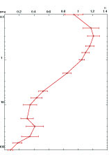
Figure 2a and Figure 2b represent the annual mean temperature and ozone content differences between solar maxium and solar minimum for a tropical latitude.
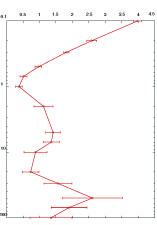
Figure 3a and Figure 3b are the annual mean temperature and ozone differences for the
zonal mean.
Figure 4 is zonal wind difference between solar maximum and solar minimum. We can see that westerly and easterly anomalies appear in the mid-high latitude each month.
In Figure 5 and Figure 6, westerly and easterly anomalies appear at latitude 70N every month.
Figure 6 shows that the anomalies shift from south to north with time.
Figure 7 shows that EP-flux anomalies direction changing every month.
The scaling factor of Fz is 125.
Conclusions
The two experiments allowed showing that the difference of the annual mean temperature and ozone amount between at the solar maximum and at the solar minimum can be noticeable in the upper stratosphere and mesosphere (Fig.2).
Over the higher latitudes however, such a difference is less clear because of the high standard deviation related to small insolation in this region in winter. Hirooka (1994) 's analysis of measurement made at 1 hPa showed a local temperature difference of 2K, while the model simulated a difference temperature of 1K. Moreover we have shown that zonal wind anomalies in the Northern Hemisphere during winter have about 2-month periodicity (Fig.5 and 6). Those anomalies appear in the mid-high latitudes and shift poleward with time from October to March.
The change in the EP-flux anomalies highlights the influence of
the solar cycle on the magnitude of the planetary waves (Fig.7).
However, the factors involving this magnitude variation are not
yet known.
A model taking the parametrization of the photodissosiation rates
of NOx, and HOx into account will be implemented in the future
to improve the results. An insight of the factors influencing
the variation of the amplitude of the planetary
waves will also be investigated.
References
Hirooka, T., Proceeding of conference in Meteorological Society
of Japan,1994
Kodera, K., J.Geophys.Res.,100,14,077-14,087, 1995
Lean, J.L., Rottman, G.J., Kyle, H.L., Woods, T.N., Hickey, J.R. and Puga, L.C., J.Geophys.Res.,102,29,939-29,956, 1997
Nicolet, M., J.Geophys.Res.,86,5203, 1981
Nicolet, M., J.Geophys.Res., in press, 1984
Takigwa, M., Takahashi, M. and Akiyoshi, H., J.Geophys.Res.,104,14,003-14,018,
1999
We thank Dr. Lean for providing 10.7cm solar flux data.
Back to
| Session 1 : Stratospheric Processes and their Role in Climate | Session 2 : Stratospheric Indicators of Climate Change |
| Session 3 : Modelling and Diagnosis of Stratospheric Effects on Climate | Session 4 : UV Observations and Modelling |
| AuthorData | |
| Home Page | |