1 Climate Research Group, Department of Atmospheric Sciences, University
of Illinois at Urbana-Champaign, 105 S. Gregory Street, Urbana,
IL 61801, USA
2 Main Geophysical Observatory, Russia
FIGURES
Abstract
Introduction
The interannual variability of many atmospheric chemical species depends on atmospheric photochemical and dynamical processes. Because these processes are not uniform throughout the atmosphere, they create a unique signature for the different atmospheric species whose lifetimes are of intermediate length (from days to a few years). Ozone and methane are such atmospheric species.
One pattern of atmospheric interannual variability that may affect these atmospheric chemical species is the Arctic Oscillation (AO), which is the variation in the intensity and position of the north-polar vortex due to an intensification of atmospheric wave activity. This pattern of variability was recognized from observed data (Kuroda, and Kodera, 1998; Kuroda and Kodera, 1999; Gong and Wang, 1999; Baldwin and Dunkerton 1999; Kawamoto and Shiotani, 2000; Wang and Ikeda, 2000) and General Circulation Model experiments (Limpasuvan, and Hartmann, 1999; Kidson and Watterson, 1999; Perlwitz et al., 2000). Here we present the interannual variability of climate and chemical species over the northern polar cap, 50°N-90°N.
Method
To study the relationship between interannual climate variability and the interannual variability of atmospheric methane and ozone we use the University of Illinois at Urbana-Champaign (UIUC) Stratosphere/Troposphere Atmospheric Chemical Transport Model (ACTM) and the UIUC Coupled Chemistry/Climate Model (UIUC CC/CM). The photochemical routine of the ACTM and UIUC CC/CM includes all of the principal gas-phase and heterogeneous reactions involved in the production and loss of chemical species (Rozanov et al., 1999, 2000). The climate part of the UIUC CC/CM also reproduces the main features of the atmospheric circulation (Yang, 2000).
Both models have a 4 degree latitude by 5 degree longitude resolution and have 24 layers from the Earth's surface to 1 hPa.
We have performed two experiments with each of these models, a control run and an experiment run. In the first pair, each run was a 15-year equilibrium simulation with the UIUC CC/CM. The control run was made with the sea surface temperature, sea ice and solar insolation specified for the current climate. In the experiment run the spectral distribution of solar radiation at the top of the model atmosphere was changed to equal that observed at solar maximum (Lean et al, 1995). In the second pair, each a 6-year transient simulation with the ACTM, the control run was made with the current observed geographical distributions of the surface sources of CO2, CH4, N2O, CFC-11 and CFC-12, taken from the NOAA/CMDL database (http://www.cmdl.noaa.gov/hats/index.html), and the surface fluxes of NOx and CO, taken from MÃ?ller and Brasseur (1995). The experiment run was made with the surface source of CFCs increasing 3% per year (WMO, 1999). In these ACTM simulations, the three-dimensional winds and temperature fields were prescribed from the UKMO reanalysis dataset for 1993-1999 (Swinbank, and Oâ?™Neill, 1994).
To define the principal modes of climate variability in the stratosphere
and troposphere over the high-latitude domain, 50°N-90°N, together
with the principal modes of the variability of ozone and methane,
we calculated Temporal Empirical Orthogonal Functions (TEOFs).
TEOF analysis allows presentation of the original time series
in terms of the sum of the product of a set of time-independent
spatial modes, ![]() , and their corresponding spatially-independent temporal eigenvectors,
, and their corresponding spatially-independent temporal eigenvectors,
![]() ,
,
![]() ,
,
where k is an atmospheric level; j is a mode of variability;![]() and
and ![]() are longitude and latitude; t is time; and
are longitude and latitude; t is time; and ![]() is the time series of quantity being investigated. Each mode j
with eigenvector
is the time series of quantity being investigated. Each mode j
with eigenvector ![]() has its unique eigenvalue
has its unique eigenvalue ![]() , which after being normalized, defines the contribution of the
corresponding mode to the total variability of the quantity. For
each model variable we analyze the first mode of its variability,
which is expressed by the first term in the summation in the above
equation,
, which after being normalized, defines the contribution of the
corresponding mode to the total variability of the quantity. For
each model variable we analyze the first mode of its variability,
which is expressed by the first term in the summation in the above
equation, ![]() . For each atmospheric pressure level, the pattern and time evolution
of the first mode may be different. In our analysis they are sorted
in increasing order of magnitude of their eigenvalues, thus the
first mode defined by the largest value of the eigenvalue. We
calculated the TEOFs for each of 24 model atmospheric pressure
levels and each month of the n-year model runs.
. For each atmospheric pressure level, the pattern and time evolution
of the first mode may be different. In our analysis they are sorted
in increasing order of magnitude of their eigenvalues, thus the
first mode defined by the largest value of the eigenvalue. We
calculated the TEOFs for each of 24 model atmospheric pressure
levels and each month of the n-year model runs.
We have mapped the magnitude of the normalized eigenvalues expressed in percent, for each quantity as a function of atmospheric pressure and month. Mapping the normalized eigenvalues of the first mode gives visual information about the atmospheric location where and month when the first mode dominates the variability. The closer the eigenvalues are to 100%, the closer the first mode is to the variabilty climatology over the corresponding time period. We have compared the climate variables' eigenvalue maps (EVMs) calculated from the model simulations and the UKMO and NCEP reanalysis datasets (http://www.sparc.sunysb.edu/html/ref_clim.html). Then we produced maps of the difference between the control and experimental runs to locate the changes in the dominance of the first mode of interannual variability for geopotential height (GPH), temperature and chemical species. Finally, we examined how the changes in solar radiation and the surface sources of CFC affected the interannual variability.
Results
For our analysis we used variables monthly means. The eigenvalue maps (EVMs) for GPH and temperature for the UIUC CC/CM control run are presented in Fig. 1 (a and b).
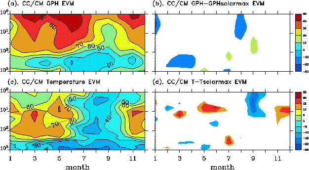
Figure 1: UIUC CC/CM EVM (%) for GPH (a) and temperature (b), and difference EVM (%) for GPH (c) and temperature (d) between control and experimental 15-year runs. In (c) and (d) the magnitudes of the differences less than 10% are masked.
For comparison, the EVMs for the NCEP and UKMO reanalysis data are presented in Fig. 2.
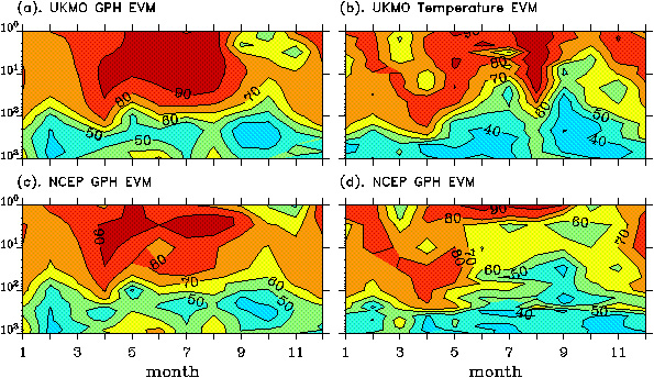
Figure 2: UKMOEVM (%) for GPH (a) and temperature (c); and NCEPEVM (%) for GPH (b) and temperature (d)
In general all three data sets show a correspondence. The main feature for the geopotential height is the strong dominance of the first mode in the stratosphere for most of the year, with exceptions in August-October for UIUC CC/CM (Fig. 1a) in the lower stratosphere and September-November for UKMO (Fig. 2a) and NCEP (Fig. 2b) in the upper stratosphere. For temperature, the UIUC CC/CM data (Fig. 1c) show a greater similarity with the NCEP (Fig. 2d) data than the UKMO data (Fig. 2c), with dominance of the first mode during January-May in the stratosphere and a reduction therein (stronger for the UIUC CC/CM) during June-October. The UKMO data (Fig. 2c) show the dominance of the first temperature mode in the stratosphere during almost the entire year.
Figures 3a and 3b are the EVMs for ozone and methane from the 15-year control run of the UIUC CC/CM. Figure 3c is the EVM for ozone from the ACTM run with the wind field prescribed from the UKMO reanalysis dataset. Comparison of Fig. 1 (a and b) and Fig. 3 (a and b) shows that in the middle and lower stratosphere the UIUC CC/CMâ?™s ozone EVM (Fig. 3a) corresponds more to the temperature EVM (Fig. 1b) than to the GPH EVM (Fig. 1a), while in the upper stratosphere the ozone EVM (Fig. 3a) corresponds more to the GPH EVM (Fig. 1a) than to the temperature EVM (Fig. 1b). The methane EVM (Fig. 3b) corresponds to the GPH EVM only in the summer months in the upper and middle stratosphere. Figure 3c shows that the EVM for ozone calculated by the ACTM without feedbacks on the circulation and temperature reveals less deviation from the climatological mean than does the ozone calculated by the UIUC CC/CM, especially in the lower stratosphere and upper troposphere.
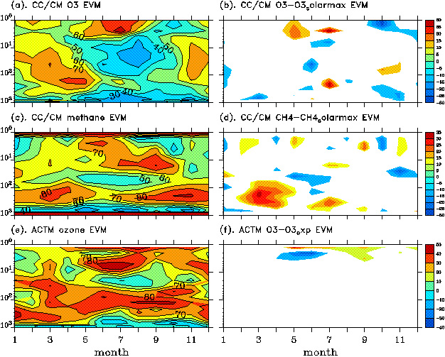
Figure 3: UIUC CC/CM EVM (%) for ozone (a) and methane (b), difference EVM (%) for ozone (d) and methane (e) between control and experimental 15-year runs; and ACTM EVM (%) for ozone and its difference EVM (%) between control and experimental 6-year ACTM runs. In (d), (e) and (f) the magnitudes of the differences less than 10% are masked
We determined the change in the EVMs for the first modes of temperature, GPH, ozone and methane resulting from the two experiments . Figures 3d and 3e show the difference between the EVMs for the control run of the UIUC CC/CM with the observed average spectrum of solar radiation and the experiment run of the UIUC CC/CM with the observed increase in solar UV radiation from solar minimum to solar maximum added to the average spectrum of solar radiation. The increased solar UV radiation influenced both the solar heating rates in atmosphere and the photolysis rates in the atmospheric chemical reactions. Figure 1 (c and d) shows the corresponding changes in the GPH EVM (Fig. 1c) and temperature EVM (Fig. 1d). Figure 3f shows the change in the ozone EVM due to the 3% per year change in surface sources of CFCâ?™s calculated by the ACTM with the UKMO reanalysis winds. On all these figures, positive values mean that the role of the first mode is diminished due to the change in boundary condition, either the solar radiation at the top of the atmosphere or the CFC source at the bottom of the atmosphere. For clarity, all changes less than 10% are not shown in the difference maps.
For the difference between the UIUC CC/CM runs (Figures 1c, 1d, 3d and 3e), the positive and negative changes in the EVM are rather significant over the entire atmosphere for all four quantities. For the ACTM runs (Fig. 3f), the changes in the ozone EVM are significant only in the upper atmosphere. For the winter atmosphere where the AO dominates the interannual variability pattern, the change in solar radiation input reduces the dominance of the first mode for GPH and methane above 10 hPa, and for all four quantities around 100 hPa.
Figure 4 shows the relation between the first mode of climate and chemical variables for January at 4 hPa and 100 hPa. It can be seen (Fig. 4a) that for this point in time and space, the positive correlation between GPH and methane is considerably increased for the UIUC CC/CM solar maximum run in comparison with its control run. This suggests that here as a result of the increase of the input solar radiation the role of planetary-wave activity for methane increased. Figure 4 (b and c) shows the variability of the first modes for GPH and methane for all 15 years. It can be seen that in the "solarmax" UIUC CC/CM run the amplitude of the first mode and the synchronicity in the variation between methane and GPH increased in comparison with control run. Both variables show a quasi-two-year oscillation in the "solarmax" run. Figure 4d shows the correlation of the first modes of methane and ozone for January at 100 hPa. It can be seen that the anti-correlation between ozone and methane in the "solarmax" experiment increased in comparison with control run. Figures 4 (e and f) show that the amplitude of the variation of both quantities in the "solarmax" run also increased. Figure 4g demonstrates a strong correlation between GPH and ozone at 100 hPa, which slightly decreases in the "solarmax" run. We conclude that the interannual variation in methane and ozone at 100 hPa has both a chemical and dynamical cause. It can be noted from Fig. 4h that an increase in the input solar radiation slightly changes the variability of GPH at 100 hPa, making it closer to the quasi-two-year period.
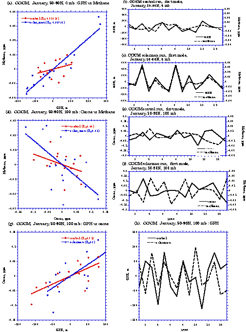
Figure 4: TheUIUC CC/CM January first mode calculated over 50°N-90°N region over 15-years model runs: (a). GPH (m) vs methane (ppm) at 4 hPa model level for the control and solar maximum experiments; (b). 15-year evolution of the first mode for GPH and methane for the control run at 4 hPa; (c). the same as (b) only for the solar maximum experiment; (d) ozone (ppm) vs methane (ppm) at 100 hPa model level for the control and solar maximum experiments; (e). 15-year evolution of the first mode for ozone and methane at 100 hPa for the control run; (f). the same as (e) for solar maximum run; (g) ozone (ppm) vs GPH (m) at 100 hPa model level for the control and solar maximum experiments; (h) 15-year evolution of the first mode for GPH at 100 hPa for the control and solar maximun experiments
Conclusions
We have studied the relationship between the interannual variability of climatic and chemical variables based on mapping the normalized eigenvalues of the first mode of their variability. We have shown that the eigenvalue maps (EVMs) allow comparison of the simulated and observed pressure-time distributions of the relative contribution of the first mode to the interannual variability. The EVMs also allow the determination of the change in the contribution of the first mode due to changes in boundary conditions at the top and bottom of the atmosphere.
From the comparison of the ACTM simulations that have no feedback on climate with the coupled climate/chemistry simulations we conclude that the former gives a greater contribution of the first mode for the ozone variability. From the coupled climate/chemistry simulations we have learned that in the upper stratosphere in January within 50°N-90°N, an increase in the input of solar radiation intensifies the relationship between the variabilities of the climatic and chemical variables.
References
Baldwin, M. P. and. T. J. Dunkerton (1999): Propagation of the Arctic Oscillation from the stratosphere to the troposphere, JGR, 104, D24, 30937-30946
Gong, D. Y. and S. W. Wang (1999): Definition of Antarctic Oscillation Index, Geophysical Research Letters ,26: (4) 459-462
Kidson, J. W., and I. G. Watterson (1999): The structure and predictability of the "high-latitude mode" in the CSIRO9 general circulation model, Journal Of The Atmospheric Sciences , 56: (22) 3859-3873 .
Kawamoto, N, and M. Shiotani (2000): Interannual variability of the vertical descent rate in the Antarctic polar vortex, Journal Of Geophysical Research-Atmospheres ,105: (D9) 11935-11946
Kuroda, Y, and K. Kodera (1998): Interannual variability in the troposphere and stratosphere of the southern hemisphere winter, Journal Of Geophysical Research-Atmospheres , 103: (D12) 13787-13799 , 1998
Kuroda, Y, and K. Kodera (1999): Role of planetary waves in the stratosphere-troposphere coupled variability in the northern hemisphere winter, Geophysical Research Letters, 26: (15) 2375-2378
Lean J., J. Beer and R. Bradley, (1995): Reconstruction of solar irradiance since 1610: Implications for climate change, Geophys. Res. Lettr., 22, 23, 3195-3198
Limpasuvan, V., and D.L. Hartmann (1999): Eddies and the annular modes of climate variability, Geophysical Research Letters , 26: (20) 3133-3136 .
Maeller, J.-F. and G. Brasseur, (1995): IMAGES: A three-dimensional chemical transport model of the global troposphere, J. Geophys. Res., 100, 16,445-16,490
Perlwitz, J, H.F. Graf, and R. Voss (2000): The leading variability mode of the coupled troposphere-stratosphere winter circulation in different climate regimes, Journal of Geophysical Research-Atmospheres , 105: (D5) 6915-6926 , 2000
Rozanov, E. V., V. A. Zubov, M. E. Schlesinger, F. Yang, and N. G. Andronova (1999) The UIUC 3-D Stratospheric Chemical Transport Model: Description and Evaluation of the Simulated Source Gases and Ozone, J. Geophys. Res.,104,11,755-11,781.
Swinbank, R. and A. O'Neill, (1994): A stratosphere-troposphere data assimilation system, Mon. Wea. Rev., 122, 686-702
Wang, J. and M. Ikeda (2000): Arctic oscillation and Arctic sea-ice oscillation. Geophysical Research Letters, 27: (9) 1287-1290 , 2000.
WMO, (1999): Scientific Assessment of Ozone Depletion: 1998
Back to
| Session 1 : Stratospheric Processes and their Role in Climate | Session 2 : Stratospheric Indicators of Climate Change |
| Session 3 : Modelling and Diagnosis of Stratospheric Effects on Climate | Session 4 : UV Observations and Modelling |
| AuthorData | |
| Home Page | |