(*) Laboratoire du Météorologie Dynamique du CNRS,
Ecole Polytechnique, Palaiseau, France
(**) Service d'Aéronomie du CNRS, Verrières les Buisson,
France
FIGURES
Abstract
Global observations from the satellites of the TIROS-N series, equipped with the HIRS-2 (High resolution Infrared Radiation Sounder) and MSU (Microwave Sounding Unit) radiometers permit the determination of atmospheric temperature profiles up to 10 hPa (about 30 km). At present time, more than 8 years of TOVS data (Jan 87 - Aug 95) have been reanalysed using the Improved Initialization Inversion (3I) developed at Laboratoire de Météorologie Dynamique. Mean layer temperatures for the layers 100-70, 70-50, 50-30, and 30-10 hPa are thus available on a day-by-day basis, and also averaged over pentads and over months, with a spatial resolution of 1 degree in latitude by 1 degree in longitude.
Comparisons between monthly-mean temperatures obtained by 3I and produced independently by the Free University of Berlin over the Northern Hemisphere will first be presented and discussed. Then, the influence of the QBO, the ENSO and the Pinatubo eruption on the temperatures will be examined.
Introduction
The study of the variability of stratospheric temperatures would ideally require homogeneous, long-recorded, high vertical resolution data. Existing observations differ in type of measurements, length of time period and time-space sampling. Data from ground-based instruments such as lidar, radiosonde, rocketsonde cover rather long periods but are not uniformly distributed around the globe; conversely, satellite data provide global coverage and uniform distribution permitting a time-space analysis of pattern variability. On the other hand the vertical resolution is much coarser.
While there is an overall agreement on a negative stratospheric temperature trend over the last 2-3 decades, the amplitude of the trend depends on what is used for its inference (WMO report, 1998). Besides, the estimation of the trend requires a precise knowledge of the influence of the solar cycle, volcanic eruptions, QBO, and ENSO which all play an important role in the stratospheric temperature variability.
The purpose of this work is to attempt to discriminate the effect of the previously-discussed factors on the variability of the stratospheric temperatures, so that a trend can be estimated. In a first step, in order to quantify the uncertainties in our dataset, comparisons between our record and the data set of the Stratospheric Group of the Free University of Berlin (FUB) obtained in a independent way are presented. Then, the response to the QBO, ENSO and solar forcings are isolated from the long-term linear trend using a multi-parameter least squares fit analysis.
Data
The data used in this study are provided by the NOAA series polar satellites, which carry onboard the TIROS-N operational Vertical Sounder (TOVS). TOVS consists of three passive vertical sounding instruments (Smith et al, 1979): the High resolution Infrared Radiation Sounder (HIRS-2), a radiometer with 19 channels in the infrared and one in the visible band, the Microwave Sounding Unit (MSU) with 4 channels operating at 55 GHz, and the Stratospheric Sounding Unit (SSU) with 3 channels near to 15 micron. HIRS-2 and MSU data for the period ranging from January 1987 until June 1995 have been reanalyzed using the 3I algorithm (e.g. Chedin et al., 1985; Scott et al., 1999) to derive in particular the vertical temperature profile from the surface up to 10 hPa. Our study makes only use of monthly mean temperatures of four atmospheric layers: 100-70, 70-50, 50-30 and 30-10 hPa. The temperatures are gridded on a regular 1deg latitude per 1 deg longitude grid.
The 8.5 year measurement period covers about 3 QBO oscillations, 2 strong ENSO events ('87 and '92, refer) and the Pinatubo eruption (June '91). It covers a maximum in the solar cycle ('88-'92); but not an entire cycle
Analysis Method
In order to isolate the response of the solar, QBO and ENSO forcings from a long-term linear trend in the monthly time series temperature data, we used a multiparameter least squares fit analysis (AMOUNTS, Adaptative Model for Unambiguous Trend Survey) developed by Hauchecorne et al., 1991; Keckhut et al. 1995 The regression model used is :
T(t) = m + St + A.trend + B.solar +C.QBO
+ D.ENSO + Nt (Eq.
1)
where for each gridpoint, T(t) is the temperature of month t, m is a constant term, St is a seasonal component which includes annual, semi-annual and terannual terms of the form:
![]()
A and B terms include an annual and semi-annual variation, in contrast to the C and D terms which take into account only the annual cycle so that the total number of parameters to be fitted is 23.
The 10.7 cm solar radio flux, well correlated with the 11-year sunspot cycle, has been taken as an indicator of solar variability. The reference QBO time series is the monthly tropical wind at 45 hPa in m/s (negative when easterly). Concerning ENSO, the standardised Southern Oscillation Index (NCEP/NCAR data) was chosen. For isolating the stratospheric warming effect due to Pinatubo eruption, analyses have been performed on the whole dataset (8.5 years) and on a reduced dataset (where the period June '91-September '93 was omitted). Finally, in equation (1), Nt is the residual term. At this first stage we assume that it is a stationary first order autoregressive process AR(1), so that
Nt = F.Nt-1 + et (Eq. 3)
where et are independent random variables with mean zero and common variance s2 . For the stationarity, we assume -1 < F < 1, where F is the autocorrelation whose positive value indicates a long-term natural variation in the time series data.
Comparisons with FUB data
FU Berlin monthly mean temperatures are available only for the northern hemisphere. They are deduced from daily analyzed temperatures for 00:00 UTC, which result from a subjective analysis, using over land the radiosonde observations and over sea the routinely-transmitted SATEMs (i.e. thicknesses derived from SSU) and assuring a backward time consistency (Pawson and Naujokat, 1997). The procedure used for performing the comparisons at a spatial resolution of 5° lat x 5° lon (which is the FUB data resolution) has been discussed in Claud et al, 1999.
Figure 1 shows the zonal mean bias (Bottom) and the standard deviation (Top) for the temperature difference 3I - FUB as a function of time (month) for the 100-50 hPa layer. The bias is found generally negative (3I less then FUB), with larger values at the end of the spring for latitudes centered at about 40 °N. However, there is some interannual variability, and the differences are on average smaller during the '92-'93 period, which are the years which follow the Pinatubo eruption. The standard deviation (Fig. 1b) is maximum for high latitudes during the winter months in relationship with the larger dynamical range of the temperatures over these areas during this period. In summer standard deviation values are more homogeneous independently of the latitudes.
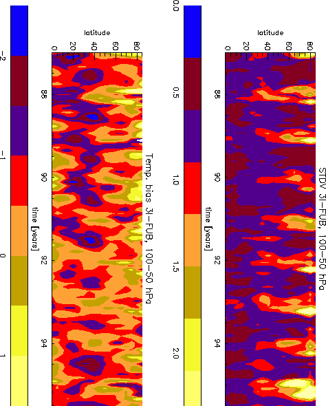
Figure 1 : Zonal mean bias (Bottom) and standard deviation (Top) for the temperature difference 3I-FUB versus time in 100-50 hPa layer
The standard deviation pattern for the 50-30 hPa and 30-10 hPa layers (not shown) is similar to that presented in Fig.1a; in the 50-30 hPa layer, the largest differences are observed in tropical and subtropical areas during wintertime.
Comparisons have also been performed separately over sea and over land showing a slightly better agreement over land, i.e. where FUB data rely mostly on radiosoundings both in terms of bias and standard deviation.
Values of the standard deviation (less than 2.5 K) and of the bias (in the range -3; 2 K) demonstrates the good quality of the data; in addition it shows the overall continuity of the satellite products (before August 91, NOAA-10 data were used, while afterwards it was NOAA12).
Characteristics of the temperature variations
The results of the regression model terms are presented for the regions where the significance is the 95%. In addition, all the results presented here have been obtained excluding the Pinatubo period.
Seasonal components
The seasonal components (not shown) exhibit, as expected, an annual signature with the amplitude decreasing with height up to 10 hPa in the extra-tropics and 30 hPa in the Tropics. In agreement with Reid (1994), a significant semi-annual signal is observed in the tropical stratosphere for the 30-10 hPa layer with two maxima in April and October.
QBO signal
It is for the highest layer (Figure 2, bottom) that the QBO signature (constant part of term C in Eq. 1), symmetrical to the equator, is the strongest, with temperatures warmer during the eastern phase of the QBO. The amplitude of this term indicates that 30-10 hPa tropical temperatures are dominated by the QBO oscillation.
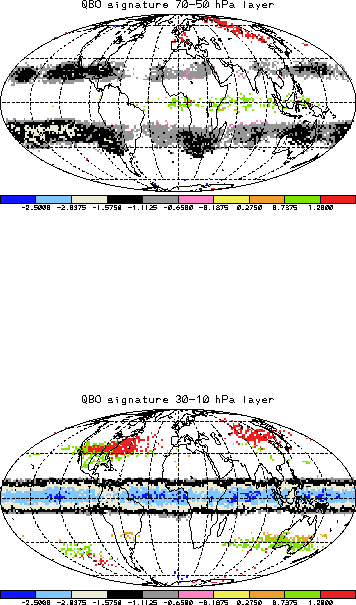
Figure 2 : Calculated latitude-longitude patterns of QBO temperature
variability in Kelvin per QBO cycle (constant part of term C in Eq. 1)
for the 70-50 (top) and 30-10 (bottom) hPa layers in the regions where
it's 95% significant.
In the 100-70 hPa layers (not shown) and 70-50 hPa, a signature is found at higher latitudes (20-30 °) in both the hemispheres and a dipolar structure at latitudes higher then 60°N, the amplitude of which depends on the terms considered in Equation 1.
No significant annual variation of the QBO term is observed.
ENSO signal
The ENSO signal (D term in Eq.1) as well as its seasonal dependence which, contrary to the QBO, is not negligible, are now examined.
Figure 3 shows the 95% significant ENSO pattern with its annual amplitude and phase for the 100-70 hPa layer (Kelvin per normalized SOI index).
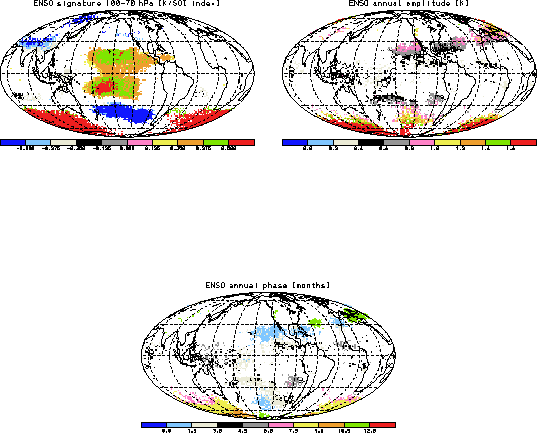
Figure 3: Top: Calculated ENSO pattern (D term in Eq. 1) for the 100-70 hPa layer in Kelvin per standardized SOI index and amplitude of annual oscillation of the ENSO pattern for the 100-70 hPa layer . Bottom: Phase of the annual ENSO oscillation [months].
The latitude-longitude structure over the globe of the ENSO term (figure 3a) consists of two positive centres symmetric to the equator and a negative one at higher latitudes in the Southern Hemisphere (at about 45° S).
The annual oscillation, whose amplitude and phase are given in figure 3b and 3c respectively, give a positive/negative contribution near to the Equator on February/July between 20°N-20°S and a reversed one (positive in August) at high latitudes in the southern hemisphere.
The ENSO effect diminishes with increasing height and vanishes above 30 hPa.
Trend and solar signal
We performed two different analyses including and excluding the solar term to avoid introducing errors due to the shortness of the period which does not include a complete solar cycle. Comparing the results we conclude that our record is far too short to isolate trend term from solar forcing because the trend and solar terms are spatially and temporally related (Randel, and Cobb, 1994).
Study of the residual term
To study the residual term we performed the statistical analysis of monthly time series data using first a simpler model which accounts for the constant, seasonal, trend and residual terms only. The idea is that the influence of the other factors (i.e. ENSO, QBO and solar cycle) on trend estimation is accounted for the residual term Nt.
Following the works of Tiao et al. (1990) and Weatherhead et al. (1998), we can evaluate the standard error of the trend estimate, in the hypothesis the residual term is AR(1). The standard error is highly dependent on the variance and autocorrelation of noise Nt. Adopting the rule that a trend is real or significantly different from zero at the 95% level if its absolute value is greater than 2 times its standard deviation, Tiao et al. and Weatherhead et al. estimated the minimum number of years of data required to detect a real trend of specified magnitude. In figure 4 (top) we show the estimated number of years necessary to detect a trend (of magnitude of 0.3% per year) plotting residual autocorrelation versus noise standard deviation for different latitudes in the 30-10 hPa layer.
Contour curves indicate the number of years of data needed to detect a 0.3% per year trend; the coloured points are the real variance sN (in percent) and F at different latitudes for the northern hemisphere; similar results are found for the southern hemisphere. The latitudinal dependence is obvious: low latitude data have positive F and lower sigma then high latitude points.
In a second experiment, the QBO term was considered (Figure 4, bottom: as expected, for low latitudes, we need less years to detect a significant trend. From this graph, we can expect to be able to determine a trend for all latitudes, once all the NOAA/TOVS (available since 1979) will be reanalyzed.
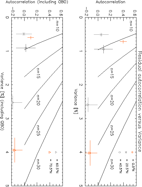
Figure 4: Residual autocorrelation versus variance [%] for points at different latitudes. Contour curves are the estimated number of years of data required to detect a 0.3% per year trend with the 95% of significance. Points are residual latitudinal average for autocorrelation and variance with their standard deviation at 5 different latitudes.
Top: using a simpler model which accounts for the constant, seasonal, trend and residual term only. Bottom: including the QBO term.
Conclusions and perspectives
TOVS data, covering the entire globe, and available for the last 2 decades permit a spatio-temporal analysis of the variability of the temperature in the stratosphere. With the least square method, it is possible to delineate the QBO and ENSO influence, and it should be possible to isolate the long term linear trend from the other terms of forcing, provided the entire data set is used.
In the future, we plan to introduce an NAO term in Equation 1. In addition, similar regression experiments will be conducted with FUB data.
References
Chedin, A., N.A. Scott, C. Wahiche, and P. Moulinier, 1985: The Improved Initialization Inversion method: a high resolution physical method for temperature retrievals from satellites of the TIROS- N series, J. Clim. Appl. Meteor, 24, 128-143.
Claud C., N.A. Scott., and A. Chedin, 1999 : Seasonal, interannual and zonal temperature variability of the tropical stratosphere based on TOVS satellite data : 1987-1991, J. Clim., 12, 540-550.
Hauchecorne, A., Chanin, M-L., and P. Keckhut, 1991: Climatology and trends of the middle atmospheric temperature (33-87 km) as seen by Rayleigh lidar over the south of France, J. Geophys. Res.,96, 15297-15309.
Keckhut, P., A. Hauchecorne, and M.-L. Chanin, 1995 : Midlatitude long-term variability of the middle atmosphere: trends and cyclic and episodic changes,J. Geophys. Res.,100, 18887-18897.
Pawson, S., and B. Naujokat, 1997 : Trends in daily wintertime temperatures in the northern stratosphere, Geophys. Res. Lett., 24, 575-578.
Randel, W.J., and J.B. Cobb, 1994 : Coherent variations of monthly mean total ozone and lower stratospheric temperature, J. Geophys. Res., 99, 5433-5447.
Reid, G., 1994 : Seasonal and interannual temperature variations in the tropical stratosphere, J. Geophys. Res., 99, 18923-18932.
Scott, N.A., A. Chedin, R. Armante, J. Francis, C. Stubenrauch, J.P. Chaboureau, F. Chevallier, C. Claud, and F. Cheruy, 1999 : Characteristics of the TOVS Pathfinder Path-B Dataset, Bull. Am. Meteorol. Soc., 80 (12), 2679-2701.
Smith, W.L., H.M. Woolf, C.M. Hayden, D.Q. Wark, and L.M. McMillin, 1979 : The TIROS-N Operational Vertical Sounder, Bull. Am. Meteorol. Soc., 60 (10), 1177-1187.
Tiao et al., 1990: Effects of autocorrelation and temporal sampling schemes on estimates of trend and spatial correlation, J. Geophys. Res., 95, 20507-20517
Weatherhead et al., 1998 : Factors affecting the detection of trends: statistical considerations and applications to environmental data, J. Geophys. Res., 103, 17149-17161.
WMO-UNEP Report, 1998: Scientific Assessment of Ozone Depletion.
Back to
| Session 1 : Stratospheric Processes and their Role in Climate | Session 2 : Stratospheric Indicators of Climate Change |
| Session 3 : Modelling and Diagnosis of Stratospheric Effects on Climate | Session 4 : UV Observations and Modelling |
| AuthorData | |
| Home Page | |