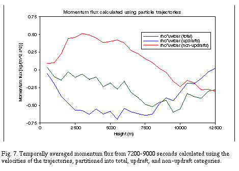
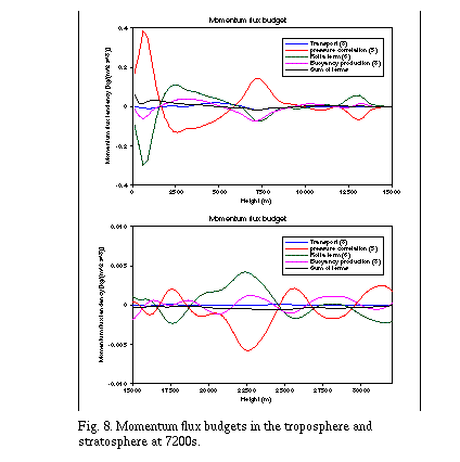
Convectively generated gravity waves have recently been identified
as a source of momentum flux that affects the mean flow in the
stratosphere and higher levels. The waves are easily identified
in the stratosphere, but difficult to discern in the troposphere
due to the much larger amplitude of the convection. In this study,
we examine a two-dimensional simulation of squall line convection
that produces vertically propagating gravity waves. Trajectory
and empirical orthogonal function (EOF) analyses are applied to
the velocity and potential temperature fields simulated by the
model, obtaining some separation of wave and convective motions.
Momentum fluxes are calculated for both convective and non-convective
motions in the troposphere, and are compared to one another. One
of the goals of this research is to develop improved parameterizations
of convectively generated gravity waves for large-scale models.
Simulation
The numerical simulation that will be analyzed here was performed
using the Advanced Regional Prediction System (ARPS - see Xue
et al. 1995). ARPS is a model with full moist physics, similar
to the model of Klemp and Wilhelmson (1978).The domain used in
the simulation was 840 km wide, and 48 km high (the upper 16 km
of which was a sponge layer). Horizontal grid spacing was 1 km,
and vertical grid spacing was 250 m. The horizontal boundaries
were periodic, and the domain moved with the storm at 16 m s-1
relative to the ground. The model was initialized with a sounding
given by Weisman and Klemp (1982), which is an analytical sounding
based on observed midlatitude squall lines that has been used
in other studies of vertically-propagating gravity waves (Fovell
et al. 1992, Alexander et al. 1995). The wind profile that was
used contains most of its 15 m s-1 of shear in the lowest 5 km
of the atmosphere, and no shear in the stratosphere.
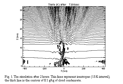
The simulation generated vertically-propagating gravity waves
that travel away from the storm, as seen in Fig. 1. The simulated
displacement of the isentropes ranged up to several hundred meters,
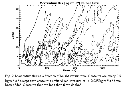
as has been observed by Pfister et al. (1993). The waves generate
momentum flux that propagates into the stratosphere as shown by
Fig. 2. The total momentum fluxes in the stratosphere are small,
but this is largely due to the fact that we are adding the contributions
of two sets of waves with comparable magnitude and opposite signs.
If the stratospheric wind became more westerly with height (for
example), then many of the easterly-propagating waves would be
absorbed within the stratosphere.
EOF Analysis
The empirical orthogonal function, or EOF, was developed by Lorenz
(1956) to develop a statistical method of weather prediction.
Although this implementation of EOFs was never used widely, EOFs
have been used to extract physically important modes of temporal
variation from large data sets. Most of these studies have focused
on finding the predominant modes for the fluctuations of fields
on planetary and synoptic scales (e.g., Kutzbach, 1967; Barnett,
1983). However, Wilson (1996) and Wilson and Wyngaard (1996) have
recently used EOFs to examine flow structures in the boundary
layer simulated by a large-eddy simulation. In these studies,
the authors found that some EOFs corresponded to gravity wave
structures, while others had the form of horizontal roll vortices.
In this section, we will examine what flow structures are uncovered
when the EOF technique is applied to convection simulated by a
mesoscale model.
The following outline of the EOF technique is similar to that
of Kutzbach (1967). Let  represent a vector of observations at M different spatial locations
taken at the nth time. If we are examining N times at which observations
are taken, then F is an M by N matrix, with the nth column corresponding
to
  . We are looking for the vector
  that is most similar to all of the
  simultaneously. The way that Kutzbach (1967) measures similarity
is by taking the normalized, squared inner product between
  and F:

.
When the above expression is maximized, each observation vector
 can be expanded as a sum of eigenvectors given by
 .
.
Each element  corresponds to the coefficient associated with the ith eigenvector
for the nth observation. As Kutzbach (1967) points out, "the coefficients
 play the same role in See .. as the coefficients in ... a Fourier series."
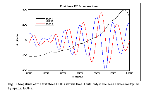
We calculated EOFs for the perturbation horizontal and vertical
velocity and potential temperature fields of the simulation at
times ranging from 3600 to 14400 seconds. Here, perturbations
are defined as deviations from the initial horizontal mean. To
normalize the potential temperature perturbations and convert
them to velocity units, they were multiplied by  , where
  is the acceleration of gravity,
  is a Brunt-Väisälä time scale of 100 s and
  is the vertically-varying basic-state potential temperature.
Since the calculation of EOFs is extremely memory-intensive, we
had to calculate the EOFs at points that covered a limited portion
of the domain (from -200 km to +200 km in the horizontal), and
with limited resolution (every 4 km in the horizontal and every
1.25 km in the vertical.) With output fields saved every 120 seconds,
this made for 91 "observations" at each point. A plot of the time-varying
coefficients for the first five EOFs is shown in Fig. 3.
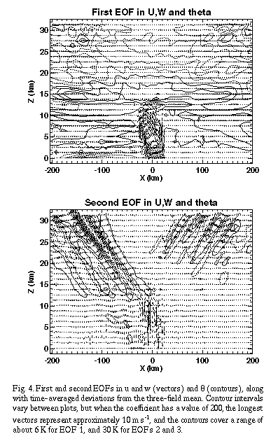
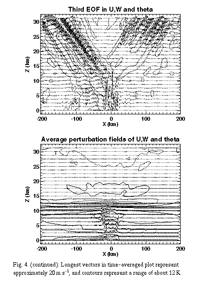
The spatial structures of the first three EOFs in u, w and ¸ are
shown in Fig. 4. The first EOF (containing 12% of the variance)
seems to be associated with the strengthening of the convection,
due to its similarity in structure to the storm averaged perturbations,
and its nearly monotonic increase in amplitude. The second and
third EOFs (containing 7% of the variance apiece) are very similar
(but slightly out of phase) in spatial and temporal structure.
They have most of their amplitude in the stratosphere (apart from
some large velocity perturbations near the region of convection),
and exhibit a phase relationship indicative of outward-propagating
gravity waves, as explained below. When the second and third EOFs
are combined in space and time (not shown), the combined mode
is similar in structure to the individual modes, except with higher
amplitude.
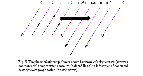
The direction that the waves in EOFs 2 and 3 are propagating can
be ascertained by examining the relative phase of vertical velocity
and potential temperature. A simplified depiction of one of these
waves is shown in Fig 5. On the left side of this wave, the upward
motion causes the air to cool, while the downward motion on the
right side of the wave is associated with warming. Since the coldest
and warmest air is to the left of the peak cooling and warming,
respectively, the wave propagates to the right.
Preliminary Conclusions
- EOF analysis can reveal a number of interesting structures in
the velocity and potential temperature fields of a numerical simulation
of convection. Some of these modes are associated with convection
in the troposphere, while others are associated with waves in
the stratosphere.
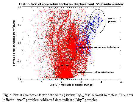
- Particle trajectory analysis obtains isolation of moist convective
updrafts within the stratosphere, which allows us to understand
how important these updrafts are to generating momentum flux,
kinetic energy and other quantities within the troposphere.
Future Work
We would like to apply the above techniques to other simulations
of convection, particularly tropical convection. Establishing
linkages between the convective momentum flux within the troposphere
and the momentum flux in the stratosphere should enable a parameterization
to be developed for large-scale models. We hope that the analysis
of the momentum flux budget and other second-moment quantities
will allow us to diagnose which physical processes are contributing
to the production of momentum flux and other quantities.
References
Alexander, M. J., J. R. Holton, and D. R. Durran, 1995: The gravity
wave response above deep convection in a squall line simulation.
J. Atmos. Sci., 52, 2212-2226.
Barnett, T. P., 1983: Interaction of the monsoon and Pacific trade
wind systems at interannual time scales. Part I: The equatorial
zone. Mon. Wea. Rev., 111, 756-773.
Fovell, R. G., D. R. Durran, and J. R. Holton, 1992: Numerical
simulations of convectively generated stratospheric gravity waves.
J. Atmos. Sci., 49, 1427-1442.
Klemp, J. B., and R. B. Wilhelmson, 1978: The simulation of three-dimensional
convective storm dynamics. J. Atmos. Sci., 35, 1070-1096.
Krueger, S. K., G. T. McLean, and Q. Fu, 1995: Numerical simulation
of the stratus-to-cumulus transition in the subtropical marine
boundary layer. Part II: Boundary-layer circulation. J. Atmos.
Sci., 52, 2851-2868.
Kutzbach, J. E., 1967: Empirical eigenvectors of sea-level pressure,
surface temperature and precipitation complexes over North America.
J. Appl. Meteor., 6, 791-802.
Lorenz, E. N., 1956: Empirical orthogonal functions and statistical
weather prediction. M. I. T. Dept. of Meteorology, Sci. Rept.
No. 1, Contract AF19(604)-1566, 49 pp.
Pfister, L., S. Scott, M. Loewenstein, S. Bowen, and M. Legg,
1993: Mesoscale disturbances in the tropical stratosphere excited
by convection: Observations and effects on the stratospheric momentum
budget. J. Atmos. Sci, 50, 1058-1075.
Stull, R. B., 1988: An introduction to boundary-layer meteorology.
Kluwer Academic Publishers. 670 pp.
Weisman, M. L., and J. B. Klemp, 1982: The dependence of numerically
simulated convective storms on vertical wind shear and buoyancy.
Mon. Wea. Rev., 110, 504-520.
Wilson, D. K., 1996: Empirical orthogonal function analysis of
the weakly convective atmospheric boundary layer. Part I: Eddy
structures. J. Atmos. Sci., 53, 1990-2013.
Wilson, D. K., and J. C. Wyngaard, 1996: Empirical orthogonal
function analysis of the weakly convective atmospheric boundary
layer. Part I: Eddy energetics. J. Atmos. Sci., 53, 801-823.
Xue, M., K. K. Droegemeier, V. Wong, A. Shapiro, and K. Brewster,
1995: ARPS version 4.0 user's guide. EC #1110, Center for Analysis
and Prediction of Storms, University of Oklahoma, Norman, OK 73109,
380 pp.
Back to
 represent a vector of observations at M different spatial locations
taken at the nth time. If we are examining N times at which observations
are taken, then F is an M by N matrix, with the nth column corresponding
to
  . We are looking for the vector
  that is most similar to all of the
  simultaneously. The way that Kutzbach (1967) measures similarity
is by taking the normalized, squared inner product between
  and F:
 .
.
 can be expanded as a sum of eigenvectors given by
 .
. corresponds to the coefficient associated with the ith eigenvector
for the nth observation. As Kutzbach (1967) points out, "the coefficients
 play the same role in
 , where
  is the acceleration of gravity,
  is a Brunt-Väisälä time scale of 100 s and
  is the vertically-varying basic-state potential temperature.
Since the calculation of EOFs is extremely memory-intensive, we
had to calculate the EOFs at points that covered a limited portion
of the domain (from -200 km to +200 km in the horizontal), and
with limited resolution (every 4 km in the horizontal and every
1.25 km in the vertical.) With output fields saved every 120 seconds,
this made for 91 "observations" at each point. A plot of the time-varying
coefficients for the first five EOFs is shown in Fig. 3.

 .
.
 .
. , we can establish the following criteria for convective updraft
motions:
 is calculated at each 120 second output time within the 7200-9000
second interval using velocity perturbations from the horizontal
means.