Previous: Measurements and Analysis Technique Next: Summary and Conclusions Up: Ext. Abst.

Analysis and Climatology

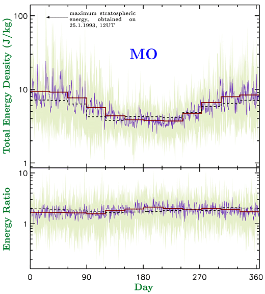
The interannual variability of the stratospheric total energy density is determined on the basis of the 10 year data set for MO and STU. Figure 2 shows this quantity and the ratio of kinetic to potential energy density for MO and both altitude ranges (AAR = 11 km and FAR = 7 km). The results for STU exhibit a qualitatively similar behaviour, but with smaller energy densities mainly in winter, and are not shown. The potenial and kinetic energy densities are given by E_pot = 1/2(g/N)²(T'/T₀)² and E_kin = 1/2(u'² +v'²), respectively, where we neglected the vertical part of the kinetic energy density.

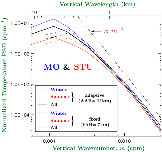
Figure 2: Interannual variability of the mean stratospheric total energy density (kinetic plus potential, top) and the ratio of kinetic to potential energy density (bottom) for MO. The blue lines represent the ten year averages over each launch date, the green shaded areas indicate the range of obtained values of the ten year period, and the red lines are the monthly averaged values (all for AAR =11 km). The dashed black lines are the monthly averaged values for FAR =7 km. Note the logarithmic scales of the ordinates.

There is a strong half-yearly trend in stratospheric energy density which can be seen in Figure 2, i.e. high stratospheric energy densities in winter and lower ones in summer. Mean values for MO are 3.8 J/kg for JJA (summer), 9.2 J/kg for DJF (winter), and 6.3 J/kg for all data. For STU the mean values are 3.4 J/kg for JJA, 7.4 J/kg for DJF, and 5.4 J/kg for all data. The ratio of kinetic to potential energy density for MO (STU) is almost constant about 1.8 (1.7) during the entire year. The stratospheric energy densities derived from the FAR analysis show qualitatively the same seasonal behaviour, but they are smaller in winter and higher in summer than those derived from the AAR analysis. Power spectral analysis, which is a technique often used in the literature (e.g. VanZandt, 1982; Allen and Vincent, 1995), shows that the energy density increases with increasing vertical wavelength, Figure 3. Since larger altitude ranges can resolve longer wavelengths, the energy density should be larger for AAR =11 km than for FAR =7 km. In winter this is the case. In summer the opposite behaviour cannot be understood with the above explanation. However, this is an artifact and comes most likely from the above mentioned tropopause effect (for the FAR analysis) that occurs more often in summer, since the tropopause in summer is higher on average (Hoinka, 1998).

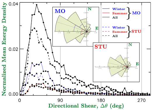
Figure 3: Power spectrum derived using FFT analysis of normalized temperature fluctuations (T'/T₀). The dotted line indicates the power law due to saturation theory ( Smith et al., 1987). The slope t of the saturated part of the spectrum is almost constant (t = 2.9), and the mean vertical wavelength is l_z =3 km (both for AAR). Note that the spectra are averaged over all data from both stations.

We now focus on the dependence of stratospheric energy density on tropospheric wind conditions, Figure 4, in order to identify the most important wave excitation mechanism north of the Alps. The tropospheric quantities are obtained between the altitudes z₀+ 1 km and z_TP - 2 km, where z₀ is the altitude above sea level of the individual station. In a first step we determine the energy weighted angular distribution of mean tropospheric wind direction (30° bins, insets in Figure 4). This gives the energetic significance of different tropospheric wind directions. In order to clarify the difference in stratospheric energy density for MO and STU, the energy densities are normalized by the sum of MO and STU. Obviously, the tropospheric wind directions in the westerly sector show high positive correlation with the stratospheric energy density. The energy weighted mean tropospheric wind directions derived from this are 287° for MO and 282° for STU. These are compatible with the wind directions from which in our region most of the active weather systems as fronts come from.

In a second step we investigate whether critical level filtering inhibits the vertical propagation of the gravity waves and thus reduces the stratospheric wave energy density. To see that, we consider the energy weighted distribution of the tropospheric directional shear, Figure 4. Again, the energy densities are normalized by the sum of MO and STU. This distribution indicates that about 80 % of the normalized energy densities are correlated with directional shears between 0° and 90° . Thus high stratospheric energy density is associated with small tropospheric directional shear in agreement with the results in Whiteway, 1999.

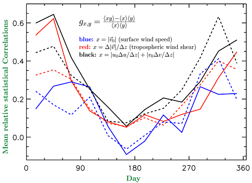
Figure 4:Energy weighted distribution of the tropospheric directional shear. Insets: energy weighted angular distributions of mean tropospheric wind directions. The dotted lines indicate the energy weighted mean tropospheric wind directions.

Finally, in a third step, we consider mean relative statistical correlations between stratospheric energy density and magnitudes derived from the tropospheric wind speed, Figure 5. They show a strong contrast between summer (correlations between -0.1 and 0.1 ) and winter (correlations between 0.2 and 0.6 ). For the winter we find positive correlation of stratospheric energy density with the surface wind speed, larger correlation with the tropospheric wind shear, and even larger correlation with both, that means the product of surface wind speed and tropospheric wind shear. Thus, since surface wind speed and tropospheric wind shear are measures for the strength of the jetstream, there is a high positive corralation in our region between jetstream strength and observed stratospheric energy density. We remark that there is a significant difference between MO and STU only for January and February referring to the correlation between stratospheric energy density and tropospheric wind shear.

Figure 5:Interannual variability of the mean relative statistical correlations . Full lines are for MO, dashed lines for STU.

Previous: Measurements and Analysis Technique Next: Summary and Conclusions Up: Ext. Abst.