• Introduction
• Instrumentation
• Analysis
• Results
• Discussion
• Conclusions and Acknowledgements
• References

FIGURES

• Figure 1
• Figure 2
• Figure 3

A climatology of cirrus clouds over the Observatoire de Haute Provence in France has been constructed from ground-based lidar measurements taken from 1997 to 1999. During this period the high-resolution lidar collected 384 nights of measurements and cirrus profiles are observed in about half of these cases. We find subvisible cirrus () constitute  of the cirrus cloud occurrences at midlatitudes and that the mean thickness of a subvisible cirrus cloud occurrence is less than 1 km.

Introduction

Cirrus clouds cover about 30 % of the earth's surface. They impact the radiation budget [Liou 1986], which in turn governs the global climate. Cirrus clouds have also been invoked as a possible surface for heterogeneous reactions that could impact ozone concentrations in the upper troposphere and lower stratosphere (UT/LS) [Borrmann et al., 1996]. Characterizing cirrus occurrences and their optical properties is critical for climate models, but there are very limited observational data. (See Penner et al. [1999] for an overview.)

In particular characterizing optically thin cirrus has been acknowledged [Rosenfield et al., 1998] as an important, albeit difficult task, for calculating heating rates. Most attention has been focused in the tropics where the largest fraction of these thin clouds has been observed [Wang et al., 1998], and the radiative effects of subvisible cirrus (SVC) are expected to be the greatest (+ 0.5 W m^-2) [Wang et al., 1996]. This prevalence of SVC in the topics has been determined using extra-terrestrial global measurements capable of detecting an optical thickness, , less than 0.03.

The objective of this study is to construct a cirrus climatology using ground-based lidar measurements over the Observatoire de Haute Provence (OHP), France. Our measurements have a high altitude resolution (75 m) and confirm the pressence of SVC at northern midlatitudes. Our study is not the first time ground-based instrumentation has observed SVC at midlatitudes. Indeed, the SVC optical thickness threshold of 0.03 was determined using midlatitude (45 ° N, 90 ° W) lidar data [Sassen et al., 1989]. Most ground-based studies of SVC have been limited in scope (e.g. see Sassen and Cho [1992]) and thus extracting climatological data from lidar work has been quite challenging. Our findings are distinctive because they are based on the most exhaustive record of ground-based cirrus observations.

Instrumentation

The Rayleigh/Mie lidar at OHP makes measurements during the night throughout the year. OHP is situated at 43.9 ° N, 5.7 ° E and at 684 m altitude. We give an overview of the instrumentation here; details can be found elsewhere [Keckhut et al., 1993,Hauchecorne et al., 1992]. A doubled Nd-YAG laser which emits a light pulse of  10 ns at 532.2 nm is operated at a repetition rate 50 Hz with an average pulse energy of 300 mJ. The lidar functions in cirrus mode between 100 - 150 nights per year.

The OHP lidar has an extensive altitude range (1 - 80 km), but the description of the detection system given here is limited to that which has been optimized for the UT/LS. The receiving telescope has an adjustable diaphragm that allows a maximum diameter of 20 cm. The altitude range for this telescope is between 1 and 25 km. The photon counting system has a 0.5 ms bin width corresponding to an altitude resolution of 75 m; the received backscatter signal is averaged over 160 seconds intervals. The lidar is operated in semi-automatic mode (i.e., signal collection is stopped only if precipitation occurs or with the onset of dawn). A typical measurement period is 6 hours. Presently the OHP lidar is not equipped with a polarizing detector, thus no information about the size or phase of the aerosols is obtained. Atmospheric temperature measurements are taken from high-resolution (Vaisala RS80) radiosondes launched from Nîmes ( 120 km east of OHP).

Analysis

A scattering ratio (SR) is calculated from the sum of Rayleigh and Mie (aerosol) scattering coefficients, (, respectively), divided by the Rayleigh backscatter coefficient:

The numerator corresponds to the raw lidar signal corrected for the background and the altitude squared dependence. The denominator is obtained using a fourth degree polynomial fit to the backscattered profile after the removal of the Mie component. When no aerosols are present, the SR equals one. Typically, for clear-sky conditions, the SR standard deviation at low altitudes (5 - 6 km) is  and increases to  at high altitudes (18 - 19 km). This rise in the standard deviation is due to the exponential decay in the signal with altitude. The minimum detectable optical depth for the OHP lidar is 1 x 10^-3.

The presence of cirrus is determined when the following two criteria are met: the SR is greater than the defined threshold (SR_t) and the cloud layer is situated in an air mass with a temperature of - 25 ° C or colder. The SR_t is defined as the sum of the nightly mean SR from 18 - 19 km plus three times the standard deviation for this altitude range. Because the SR_tis defined for each nightly determination, it is sensitive to the signal to noise of the particular observation. The - 25 ° C threshold, as determined from the radiosondes, has been recognized (Heymsfield, private communication) as an indicator of cirrus. Cirrus occurrence frequencies are calculated from the number of cirrus occurrences divided by the total number of measurements.

An optical thickness for a cirrus cloud is calculated from the integral of the extinction coefficient, , :

where z_min and z_max represent the minimum and maximum cirrus altitude, respectively. Using the SR and the phase function, ), we can derive the relationship used to calculate the optical thickness of cirrus:

where,  = Rayleigh backscattering cross section,  =  n_air(z), and n_air(z) = density of air, as calculated by the MSIS-E-90 atmosphere model [http://nssdc.gsfc.nasa.gov/space/model/models/msis.html]. A phase function of 18.2 sr [Platt and Dilley, 1984] is used, and_Rayleigh (532 nm) = 5.7 x 10^-32 m² sr^-1. No corrections for multiple scattering are made.

Results

From 1997 to 1999 the lidar system made 384 nights of measurements. As seen in Figure 1, cirrus clouds are observed in half of the cases (54 %). The cirrus occurrence frequencies for spring, summer, winter, and fall are 57 %, 42 %, 57 %, 60 %, respectively.

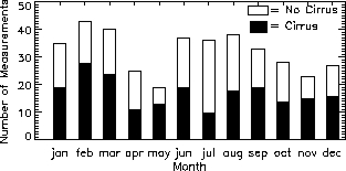
Figure 1: A histogram of the number of cirrus occurrences and the total number of nightly measurements from 1997 - 1999 as a function of month.

Figure 2 shows the location of the cloud top heights for 1998 in relation to the tropopause; altitudes that correspond to - 25 ° C are also presented in the plot. A significant portion, 43 %, of the cirrus cloud top heights are within 0.5 km of the tropopause. In Figure 2 one sees, even with the daily variability of the tropopause height, the cirrus cloud tops tend to consistently track the tropopause. We use the WMO's definition of the tropopause (the altitude where the temperature lapse rate decreases to 2 K km^-1 for at least 2 km). All temperatures are obtained from the radiosondes. Results for 1997 and 1999 are similar.

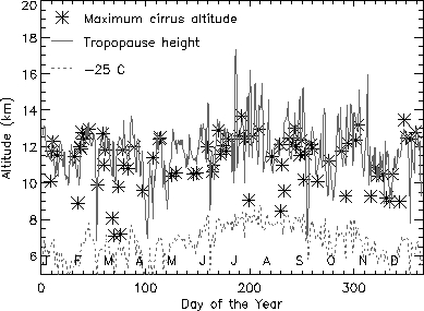
Figure 2: A profile of cirrus cloud top heights for 1998. Stars denote the maximum cirrus altitude, the solid line is the tropopause height and the dotted line marks altitudes that corresponds to - 25  C. The tropopause and - 25  C altitudes are determined from radiosondes measurements.

Table 1 summarizes the statistics for the cirrus cloud occurrence frequency for individual layers and their total thickness for the three years studied. A separation of 3 channels (corresponding to 225 m) is needed for a new layer to be declared. The mean cirrus thickness is 1.4  km and centered at 10.0  km, while the SVC are markedly thinner (0.8  km) but are located in the same region (10.4  km).

We present the optical thicknesses as a function of season in Figure 3; the results are binned on a log scale to better perceive the cases of very optically thin clouds. The SVC cloud occurance percentages for spring, summer, fall, and winter are 23 %, 18 %, 21 %, 25 %, respectively. When the mean for all three years is taken, cirrus with optical depths between 0.03 and 0.1 are the most prevalent. This pattern is similar for the annual results, except for 1998 where cirrus with optical thickness between 0.01 and 0.03 are as frequent than those between 0.03 and 0.1. The SVC cloud occurance varied from year to year, 22 % (1997), 27 % (1998), 17 % (1999).

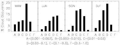
Figure 3: Histograms of cirrus seasonal optical thicknesses binned on a log scale. The first letter of each month is given in the upper left. Lettering along the absissa corresponds to optical thickness intervals, which are given above. 

Discussion

The OHP data set offers a unique perspective on cirrus clouds at northern midlatitudes. Unlike campaign data or satellite observations, the lidar measurements presented here were systematically taken over the period of three years, with excellent altitudinal and temporal resolution. Analysis has revealed many optically thin and SVC events, with the latter composing 23 % of the mean optical thicknesses.

Certain considerations must be taken into account when analyzing the OHP lidar data. With the ground-based lidar technique it is not possible to make measurements when there are opaque/precipitating clouds. Consequently it is possible that our statistics may be biased, especially the number of cirrus occurrences in the optical depth range of 0.3 - 1.0, category F in Figure 4. Generally at OHP there are only  50 nights where such conditions preclude the collection of data.

In our analysis we have made several reasonable assumptions. In the calculation of the optical thickness, we have assumed  of 18.2 sr from Platt and Dilley [1984]. This value was taken from lidar measurements (1978 - 1980) in the southern hemisphere and is estimated to have an error of 20 %; thus, this is the lower limit for the error of our calculated optical thickness. Another possible source of uncertainty is the temperatures measurements. Besides possible systematic errors of the sondes, there is the distance ( 120 km) between Nîmes and OHP. Two sondes are launched per day from Nîmes, one at noon and another at midnight (universal time). For this work we used the latter sonde, which typically temporally coincided with the lidar measurements. The temperature determinations of the Nîmes' sondes are more accurate than the Raman lidar technique [Hauchecorne et al., 1992]. For the optical thickness measurements, the sondes were used to determine the - 25 ° C threshold. If any part of the cloud layers was located at or above the corresponding - 25 ° C altitude, then the entire cloud was included in the calculation of the optical thickness. Hence, any errors in the temperature measurements would only slightly affect the optical thickness determinations. Finally, there have been differing ice threshold temperatures quoted for midlatitude cirrus [Heymsfield and Platt, 1984,Roscow et al., 1996,Riedi et al., 1999]. We conducted a reanalysis of our data using a threshold temperature of - 40 ° C. This change had a minimal effect on our results (e.g., an augmentation of only 2 % for SVC occurrences).

Conclusions

Our findings of a SVC occurrence frequency of  centered near 10 km confirm the existence of SVC at northern midlatitudes. Comparing these findings with the climatological results from the SAGE II instrument, which unlike other instruments such as HIRS, is very sensitive to optically thin cirrus (), we find excellent agreement with Wang et al. [1996] zonal average cirrus cloud occurences at 44 ° N. The high altitudinal resolution of the lidar measurements show that the mean thickness of a SVC event is less than 1 km with the distribution skewed towards much thinner layers ( are less than 0.4 km) and that cirrus cloud tops often occur at the tropopause. With nearly 2300 hours of measurements, this is the most extensive lidar study of cirrus available. These results help provide detailed cirrus climatological information that is needed to accurately model the effect of these clouds on the radiation budget.

Acknowledgements: This work was supported by Snecma and the Université Paris 6 under grant #940480. The authors also gratefully acknowledge the technical support team at OHP.

Bibliography

Borrmann et al., 1996

Borrmann, S., S. Solomon, J.E. Dye, and B. Luo, The potential of cirrus clouds for heterogeneous chlorine activation, 23, 2133-2136, 1996.

Hauchecorne et al., 1992

Hauchecorne, A., M.-L. Chanin, P. Keckhut, and D. Nedeljkovic, LIDAR monitoring of the temperature in the middle and lower atmosphere, App. Phys., B55, 29-34, 1992.

Heymsfield and Platt, 1984

Heymsfield, A.J., and C.M.R. Platt, A Parameterization of the particle size spectrum of ice clouds in terms of the ambient temperature and the ice water content, J. Atmos. Sci., 41, 846-855, 1984.

Jensen et al., 1999

Jensen, E.J., W.J. Read, J. Mergenthaler, B.J. Sandor, and L. Pfister, High humidities and subvisible cirrus near the tropical tropopause, 26, 2347-50, 1999.

Keckhut et al., 1993

Keckhut, P., A. Hauchecorne, and M.-L. Chanin, A critical review of the database acquired for the long-term Surveillance of the middle atmosphere by the French Rayliegh lidars, J. Atmos. Ocean., 10, 850-867, 1993.

Liou 1986

Liou, K.-N., Influence of cirrus clouds on weather and climate processes : A global perspective., Mon. Weather Rev., 114, 1167-1199, 1986.

Penner et al., 1999

Penner, J.E., D.H. Lister, D.J. Griggs, D. J. Dokken, and M. McFarland, Aviation and the Global Atmosphere: Special Report of the Intergovernmental Panel on Climate Change, Cambridge University Press, Cambridge, 1999.

Platt and Dilley, 1984

Platt, C.M.R., and A.C. Dilley, Determination of the cirrus particle single-scattering phase function from lidar and solar radiometric data, App. Opt., 23 (3), 380-386, 1984.

Riedi et al., 1999

Riedi, J., P. Goloub, R. Marchand, and H. Chepfer, Cloud thermodynamic phase from POLDER/ADEOS: Comparison with millimetre wave radar measurements and synoptic weather reports, In Proceedings of the Europto Conference on Satellite Remote Sensing of Clouds and the Atmosphere IV, 1999.

Roscow et al., 1996

Roscow, W.B., A.W. Walker, D.E. Beuschel, and M.D. Roiter, International Satellite Cloud Climatology Project (ISCCP),Documentation of new cloud datasets, World Climate Research Program (ICSU and WMO),Tech. Doc. WMO/TD 737, World Meteorol. Org., Geneva, 1996.

Rosenfield et al., 1998

Rosenfield, J.E., D.B. Considine, M.R. Schoeberl, and E.V. Browell, The impact of the subvisible cirrus clouds near the tropical tropopause on stratospheric water vapor, 25, 1883-1886, 1998.

Sassen and Cho, 1992

Sassen, K., and B.S. Cho, Subvisible-thin cirrus lidar dataset for satellite verification and climatological research, J. Appl. Meteor., 31, 1275-1285, 1992.

Sassen et al., 1989

Sassen, K., M.K. Griffin, and G.C. Dodd, Optical scattering and microphysical properties of subvisible cirrus clouds, and climatic implications, J. Appl. Meteor., 28, 91-98, 1989.

Wang et al., 1996

Wang, P.-H., P. Minnis, M.P. McCormick, G.S. Kent, and K.M. Skeens, A 6-Year climatology of cloud occurrences frequency from Stratospheric Aerosol and Gas Experiment II observations (1985-1990), 101, 29407-29429, 1996.

Wang et al., 1998

Wang, P.-H., P. Minnis, M.P. McCormick, G.S. Kent, G.K. Yue, D.F. Young, and K.M. Skeens, A study of the vertical structure of tropical (20 S-20 N) optically thin clouds from SAGE II observations, Atmos. Res., 47-48, 599-614, 1998.