S P A R C Stratospheric Processes And their Role in Climate A project of the World Climate Research Programme Home Initiatives Organisation Publications Meetings Acronyms and Abbreviations Useful Links

Report on the Assessment of Stratospheric Aerosol Properties: New Data Record, but no Trend

Larry W. Thomason, NASA Langley Research Center, USA (l.w.Thomason@larc.nasa.gov)
Thomas Peter, Swiss Federal Institute of Technology, Switzerland (Thomas.Peter@ethz.ch)

Contributors to this work have been the Chapter Leads: S. Bekki (France), H. Bingemer (Germany), C. Brogniez (France), K. Carslaw (UK), T. Deshler (USA), P. Hamill (USA), B. Kärcher (Germany), J. Notholt (Germany), E. Weatherhead (USA), D. Weisenstein (USA), plus many others colleagues

Introduction

Assessments of stratospheric ozone have been conducted for nearly two decades and have evolved from describing ozone morphology to estimating ozone trends, and then to attribution of those trends. The stratospheric aerosol has only been integrated in assessments in the context of their effects on ozone chemistry and has not been critically evaluated itself. As a result, SPARC has sponsored the Assessment of Stratospheric Aerosol Properties (ASAP). Initially, we expected the assessment to consist primarily of an evaluation of available stratospheric aerosol measurements, however, it rapidly became apparent that the lack of previous groundwork made a more expansive effort worthwhile. As a result, the scope of ASAP expanded to include 5 primary components referring to stratospheric aerosols: (1) Processes, (2) Precursors, (3) Measurements, (4) Trends, and (5) Modelling. Herein, we will describe the contents of these sections beginning with some of ASAP’s key findings.

Key Findings

• Unlike gas species, aerosol cannot be characterized by a single quantity but has a size distribution and composition. The vast bulk of existing data does not comprise a complete measurement set and as a result many parameters required for scientific or intercomparison purposes are derived indirectly from the base measurement. This is true for space-based measurements where only bulk extinction is measured but also true in degree for most ground-based and in situ systems. The fact that each system measures a different set of parameters greatly complicates almost every stage of measurement comparisons.
• Space-based and in situ measurements of aerosol parameters tend to be consistent following significant volcanic events like El Chichon and Pinatubo. However, during periods of very low aerosol loading, this consistency breaks down and significant differences exist between systems for key parameters, including aerosol surface area density and extinction.
• Since the beginning of systematic stratospheric aerosol measurements there have been three periods with little or no volcanic perturbation, though only the period from 1999 onwards can be confidently identified as free of volcanic aerosols. The other periods (late 1970’s and late 1980’s) are too short in duration to evaluate, given the complex variability observed. The period in the 1980’s seems likely to have not reached a stable non-volcanic level. Trends derived from the late 1970’s to the current period are likely to completely encompass a value of zero.
• There is general agreement between measured OCS (carbonyl sulfide) and modelling of its transformation to sulfate aerosol, and observed aerosols. However, there is a significant dearth of SO₂ measurements, and the role of tropospheric SO₂ in the stratospheric aerosol budget - while significant - remains a matter of some guesswork. In addition, it is not well understood whether decreasing global human-derived SO₂ emissions or increasing emissions in low latitude developing countries, such as China, dominate the human component of SO₂ transport across the tropical tropopause.
• While the actual removal of aerosol from the stratosphere to the troposphere is predominantly associated with tropopause folds, sedimentation plays an important role in the vertical redistribution of aerosol throughout the stratosphere.

Chapter 1: Processes

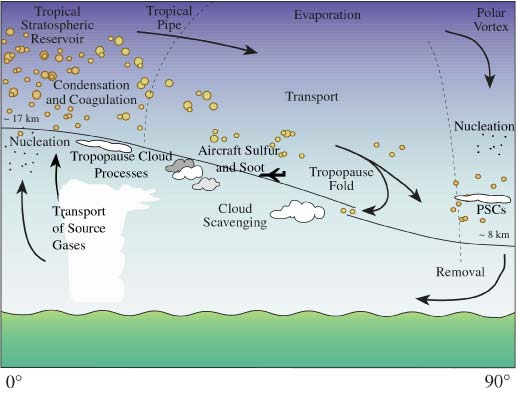
The aerosol processes section highlights the lifecycle of stratospheric aerosol (Figure 1) that involves processes of precursor gas and aerosol input to the stratosphere through the tropical tropopause, the transport and transformation of the aerosol within the Brewer-Dobson circulation, and the removal of aerosol in air traversing the extra-tropical tropopause and through gravitational settling. The non-volcanic stratospheric aerosol is formed primarily through binary homogeneous nucleation of sulfuric acid and water in rising air masses close to the tropical tropopause (e.g., Brock et al., 1995). The aerosol in the tropical regions is rapidly transported zonally with the mean stratospheric winds, while the transport is restricted meridionally by the transport barrier of the tropical pipe in the 15°-30º latitude range. This reduced transport is most effective at altitudes between about 21 and 30 km and poleward transport at lower altitudes is more rapid. After a volcanic eruption the transport barrier of the “leaky tropical pipe” leads to the build-up of a tropical reservoir of aerosol mass, first described by Trepte and Hitchman (1992). This is also reflected in Figure 2, where 1992 is the year after the eruption of Mt. Pinatubo.

Figure 1. Schematic of the stratospheric aerosol lifecycle (from Hamill et al., 1997).

Figure 2. HALOE 5.26 mm aerosol extinctions as a function of latitude and altitude for the month of July in 1992, 1994 and 1997. White areas represent missing data and lines indicate average tropopause height. Measurements identified as cirrus were removed, resulting in the absence of data below the tropopause.

The aerosol in the air masses transported into the mid and high latitudes continues to evolve through microphysical processes, such as evaporation at the upper edge of the aerosol layer and nucleation/re-condensation during descent. The air descends diabatically to the lowermost stratosphere where it can eventually be removed in the troposphere through quasi-isentropic transport of the air in tropopause folds that is the dominant removal mechanisms for stratospheric aerosol. Furthermore, throughout the lifetime of the aerosol, gravitational settling adds to the removal of these particles. Due to the long lifetime of the particles, their sedimentation velocities (~ 100 m/month for particles with 0.1 mm radius and strongly growing for larger ones) cannot be neglected. Additional removal occurs over the poles when the sulfuric acid particles serve as sites for polar stratospheric cloud (PSC) particle formation. Some PSC particles composed of nitric acid hydrate or ice can grow to several microns in diameter and sediment rapidly to the tropopause, taking included sulfuric acid particles with them. Observations clearly show the seasonal reduction in polar aerosol mass following periods of PSCs.

Chapter 2: Stratospheric Aerosol Precursors

The direct gaseous precursor for the stratospheric aerosol sulfate is sulfuric acid (H₂SO₄). With the exception of sporadic direct injections from volcanic eruptions, stratospheric H₂SO₄ originates primarily from OCS photolysis and in situ oxidation of SO₂, OCS and other reduced sulfur gases reaching the stratosphere including DMS (CH₃SCH₃), H₂S, CH₃SH, and CS₂. Since these species originate at the Earth’s surface, they are reliant on deep convection events above the continents (particularly in the tropics) to reach the lower part of the tropical transition layer (TTL). In the TTL, air carrying the sulfur compounds is quasi-horizontally transported over wide distances and eventually ascends into the stratosphere. The largest emissions of sulfur-containing compounds at the surface are SO₂ followed by DMS, H₂S, CH₃SH and OCS and CS₂. It is now believed that OCS and SO₂ are the main precursor gases for the formation of the stratospheric aerosol layer. Although the emissions of OCS are much smaller than those of SO₂ and DMS, its long lifetime allows it to reach the stratosphere. Conversely, SO^₂ can reach the TTL despite having a short lifetime in the troposphere due to rapid transport of air masses by deep convection to the bottom of the TTL. The composition of the TTL is presently not fully characterized with respect to the sulfur containing gases and radicals. On the whole, the knowledge of the seasonal and longitudinal variability of SO₂ and HO_x in the TTL is very limited.

The long-term sulfur flux into the stratosphere is expected to show some variability. First, the long-term trend of OCS, as measured by remote sensing techniques, is found to be about - 0.25%/y throughout the last 20 years. Second, the emission patterns of SO₂ have changed throughout the last decades. Long-term observations of SO₂ have been performed in situ at numerous locations. While the anthropogenic emissions in the Northern Hemisphere have decreased, emissions in Asia, China and the tropical biomass burning have increased. It is not clear to what extent these processes might compensate each other. In addition, the oxidation capacity (OH and HO_x concentrations) in the upper tropical troposphere has changed within the last decades. Since the main sink of SO₂ is its reaction with OH, changes in the OH concentration have a strong impact on the SO2 burden. Furthermore, recent studies indicate that the OH concentration within the TTL is by a factor 2-4 higher than previously assumed.

Chapter 3: Aerosol Measurement Systems

Stratospheric aerosol measurements systems were broadly divided into two groups. One group consists of systems with long continuous records, such as the Stratospheric Aerosol and Gas Experiment (SAGE) series and the Halogen Occultation Experiment (HALOE) space-based systems, the balloon-borne University of Wyoming Optical Particle Counter (OPC), and lidar systems like that at Garmisch-Partenkirchen, Germany. The other set consists of either episodic measurements like FCAS (Focus Cavity Aerosol Spectrometer) and FSSP-300 (Forward Scattering Spectrometer Probe) which are deployed primarily as a part of field campaigns like the SAGE III Ozone Loss Validation Experiment (SOLVE), or of shorter term space-based measurements like the Cryogenic Limb Array Etalon Spectrometer (CLAES). For ASAP, we focused on the former group.

HALOE and SAGE, and also the Polar Ozone and Aerosol Measurement (POAM III), make use of the solar occultation technique to measure atmospheric transmission along the line of sight between the spacecraft and the Sun along paths that pass through the atmosphere (hence the Sun, relative to the instrument, is being occulted or obscured). This technique is well suited for situations in which horizontal inhomogeneity is not a significant concern and where the optical depth is relatively low, features which are generally characteristic of the stratosphere. Using this strategy, HALOE (1991-present) makes aerosol extinction measurements in the infrared at 2.45, 3.40, 3.46, and 5.26 mm. The SAGE series of instruments consists of three instruments: the Stratospheric Aerosol Measurement (SAM II; 1978-1993), SAGE (1979-1981), and SAGE II (1984-present). All SAGE series instruments operate in the visible/near infrared and measure aerosol extinction at one or more wavelengths including one close to 1000 nm for all instruments.

The OPC, a balloon-borne system, was originally designed in the 1960s [Rosen, 1964] and has been routinely launched from Laramie, Wyoming (USA) since 1971. Given its portability it has also been extensively launched from Antarctica and was also launched from Lauder, New Zealand for several years during the 1990s and is frequently deployed during field campaigns, such as SOLVE (2000) and SOLVE II (2003). The instrument, a white light counter measuring aerosol scattering at 25° (prior to 1989) or 40°(1989 onwards) in the forward direction, measures particles one at a time and uses Mie scattering theory to convert from brightness to particle size in 2 to 12 size bins and from 0.15 to either 2.0 or 10 mm [Hofmann and Deshler, 1991; Deshler et al., 2003]. A particle size distribution is derived by fitting either a single or bi-modal log-normal to the binned data.

Chapter 4: Aerosol Measurement Record

Derived quantities like Surface Area Density (SAD) and effective radius are derived from SAGE data using a technique similar to that in Thomason et al. [1997]. The primary change from the previous version was the use of error bars to weight the measurements. For HALOE data, derived quantities like SAD are determined using the method described in Hervig et al. [1998]. Relative to versions prior to 2002, the sulfate refractive index data has been updated to that of Tisdale et al. [1998] from that of Palmer and Williams [1975]. The change resulted in an reduction of ~ 25 % in SAD from the previously archived data set. Both SAGE and HALOE data sets have identified and eliminated obvious occurrences of clouds.

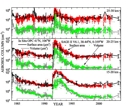
An endemic problem with these data sets becomes obvious when we attempt to do a critical comparison. Since none of these systems measure the same aerosol attributes and thus the comparisons are dependent on the robustness of the conversions as the quality of the basic measured quantities themselves. This is well illustrated by measurements of SAD in Figure 3. Here we see that comparisons of SAD between SAGE II and the OPC are typically in reasonable agreement during high aerosol loading, such as that following the Pinatubo eruption of 1991. On the other hand, when aerosol loading is low (either at high altitudes or at lower altitudes in the later 1990’s or 2000’s), SAGE II SAD is biased low by as much as a factor of 2 relative to the OPC values. This is not unexpected since low aerosol loading is also associated with generally smaller aerosol sizes. Measurements made at visible/near infrared wavelengths are primarily driven by scattering and increasingly insensitive to particles smaller than 0.1 mm. At that point, even if the extinction measurements themselves remain robust, the derived SAD becomes highly dependent on how the derived algorithm ‘chooses’ to fill the part of the size distribution that is effectively invisible. Since the SAGE II algorithm tends to put relatively little SAD in the smaller particle sizes, the bias and its sign is not unexpected.

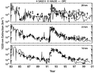
Figure 3. History of five kilometer column densities of aerosol surface area and volume in the northern mid latitudes, 1984-2004. The solid lines with intermittent error bars (±40 %) are from lognormal size distributions fit to ~ 200 aerosol profiles from balloon-borne in situ measurements above Laramie, Wyoming. Coloured symbols are SAGE II V6.1 estimates of surface area and volume from the SAGE II web site for all measurements between 38 and 44°N with no restriction on longitude.

Comparisons of HALOE and OPC extinction derived for SAGE measurements at 1020 nm are shown in Figure 4. As in the case for SAD, the agreement is quite reasonable for elevated extinction. However, in this case, when extinction drops toward non-volcanic levels a systematic bias particularly between SAGE II and the OPC values (that approaches a factor of five by the end of the period) is evident, even though the aerosol levels themselves are thought to be well within the dynamic range of both instruments. HALOE generally agrees better with SAGE II during this period but occasionally agrees better with the OPC values. The bias is in the opposite sense of the SAD bias (SAGE II greater than the OPC for extinction). Interestingly, comparisons at the shorter wavelengths are considerably better than those at 1020 nm and would imply a difference in the larger end of the aerosol size distribution between the OPC and that implied by the SAGE II measurements. Generally, SAGE II 1020 nm extinction measurements are consistent with those of POAM III and other members of the SAGE series [Thomason and Taha, 2003] and, thus, not an outlier. Such large differences in extinction values also reduce our confidence in our conclusions regarding the differences between systems in other quantities like SAD and additional work in this area is required.

Figure 4. Time series at three altitudes over Laramie of aerosol extinction at 1020 nm. SAGE II (‡) measurements are compared to extinctions calculated from OPC (-) and HALOE (á) size distributions. HALOE and SAGE II measurements between 41°N and 42°N latitude and 245°E and 265°E longitude were used. Vertical bars on the occasional SAGE II measurement indicate ± 50 %. The SAGE II uncertainties are less than this, and these bars serve only to add perspective. This time series is comprised of 68 SAGE II, 178 OPC and 31 HALOE measurements.

Chapter 5: Trends

For trend analysis, we decided to focus on the primary measured quantities of the measurement systems: extinction at 1000 nm for the SAGE series, the 0.15 and 0.25 mm bins for the OPC, and integrated stratospheric backscatter for long record lidar systems at Garmisch-Partenkirchen (Germany), Mauna Loa (USA) and Hampton (USA). It is not possible to evaluate trends in the stratospheric aerosol in the same way that trends are computed for species like ozone or water vapour due to volcanic impacts that have caused perturbations as large as a factor of 1000 at some altitudes and locations. As of this writing, this analysis has not been completed and the following discussion is still preliminary.

With the long recovery time from major events and the observed complex seasonal and quasi-biennial components to aerosol variability, stable, multi-year periods are necessary to confidently identify volcanically perturbed periods. Three time periods have been considered as candidates for non-volcanic periods. Two of these, the late 1970’s and late 1980’s/early 1990’s are of short duration and are difficult to use. The third period starts no later than 1999 and continues until late 2002 when eruptions by Ruang (Indonesia) and Reventador (Ecuador) at least temporarily ended the latest quiescent period. The late 1980’s period also appears unlikely to qualify as background since particularly the tropics exhibit an uninterrupted decrease from the El Chichon/Nevado del Ruiz eruptions of 1982 and 1985 [Thomason et al., 1997]. Finally, differences between the 1970’s (despite concerns regarding its use) and the 2000’s are small and it seems likely that the uncertainties in any derived trend will easily include zero.

Chapter 6: Modelling

The overall object of the ASAP modelling investigation was to determine whether transport of sulfur compounds (primarily SO₂ and OCS) from the troposphere and known physical processes can explain the distribution and variability of the stratospheric aerosol layer. Models, since they encompass the knowledge of coupled aerosol processes, are the primary tools to test our quantitative understanding of processes controlling the formation and evolution of the aerosol layer. As a result, comparisons between models and observations form the core of this study. The models participating in this effort were developed for modelling stratospheric aerosol and include AER (D. Weisenstein), CNRS (S. Bekki), LASP (M. Mills), MPI (C. Timmreck), and ULAQ (G. Pitari). These models are well-established 2-D and 3-D aerosol-chemistry-transport models that contain standard chemistry including that for sulfur, but they differ in their implementation for aerosol formation and evolution as well as in other components, such as in their handling of the tropopause boundary conditions.

Comparisons of the models to precursor gas measurements are generally promising. In particular, agreement among the models and measurements of OCS in the tropics are within the error bars. This is reassuring since this region is where tropospheric sources gases enter the stratosphere and where the major chemical loss of OCS occurs. The agreement between models and observations remains fairly good at other latitudes, though the models show more variability among themselves. For SO₂ in the non-volcanic stratosphere, the models are mainly compared against one another since the only observation of SO₂ under non-volcanic conditions comes from a single ATMOS profile from 1985 [Rinsland, 1995] and, therefore, its distribution is not well known. For this profile, the models do not agree well except LASP above 33 km. The models tend to agree among themselves between 20 and 30 km in the tropics, however, model differences in SO₂ much like those for OCS are much larger at higher latitudes most likely due to differences in transport. Model-computed aerosol extinctions generally agree with SAGE II and HALOE observations in magnitude and in latitudinal gradients during low aerosol loading periods. This is true above 20 km where the models themselves also tend to agree, but to a lesser degree below 20 km where some substantial divergence between the models themselves can be observed. Compared to SAGE II measurements below 20 km, the model 525 nm extinctions tend to straddle the observations while the model extinctions at 1020 nm tend to underestimate the observed extinction. This suggests that the models have redistributed some of the aerosol from larger to smaller sizes relate to that suggested by the observations. Above 20 km, the agreement between the models and SAGE II-derived SAD is comparable to the agreement found for extinction. Below 20 km, the SAGE II-derived values are substantially smaller than those computed from the models. Part of this is probably due to limitations in converting from extinction to SAD using SAGE II observations (as discussed above) but may be exacerbated in these comparisons by deficiencies in the models’ lower stratospheric size distribution.

ASAP Data Archive

Data sets that comprise the basis for the data analysis will be archived at the SPARC Data Center (http://www.sparc.sunysb.edu/) including altitude/latitude gridded fields of aerosol extinction and derived quantities for the SAGE series and HALOE. Data sets used in the trend analysis will also be available at this location. In addition, links to additional sources of aerosol data that appear within this report will be included. Also, at least the SAGE data sets will be available remapped to equivalent latitude and potential temperature.

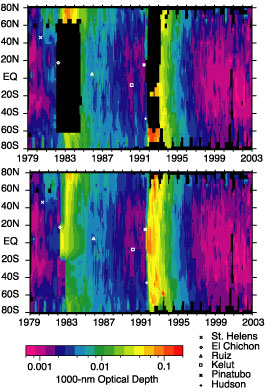
A final product that will be available is a ‘gap filled’ data set for the period 1979 through 2002 based on the SAGE record. Gaps exist between the June 1991 eruption of Mt. Pinatubo and the end of 1993 due to instrument saturation and between November 1981 and October 1984, when global space-based aerosol extinction measurements were not available. To fill the missing values, we have used aerosol backscatter profile measurements from sites at Camaguey (Cuba), Mauna Loa, Hawaii (USA), and Hampton, Virginia (USA) and backscatter sonde measurements from Lauder (New Zealand). This period encompasses the El Chichon eruption and the onset of the Antarctic ozone hole and is, therefore, of particular interest. Beginning in April 1982 and through the beginning of SAGE II observations in 1984, we have used a composite of data consisting of SAM II, the NASA Langley 48-inch lidar system, and lidar data from the NASA Langley Airborne Lidar System. Data from this later data set has only been partially recovered for the 1982 to 1984 period. Figure 5 shows the stratospheric aerosol optical depth for the 1979-2002 period using the gap-filled data product. When more of the airborne lidar data and particularly the revised aerosol product from the Solar Mesospheric Explorer (1981-1986) become available additional work on the El Chichon period will be profitable.

Figure 5. SAM II, SAGE and SAGE II stratospheric aerosol optical depth at 1000 nm from 1979 through 2002. Profiles that do not extend to the tropopause are excluded from the analysis leading to significant regions of missing data following the eruptions of El Chichón and Mt. Pinatubo in 1983 and 1991. Upper panel: original data. Lower panel: after gap-filling using auxiliary measurements (see text).

References

Brock. C.A., et al., Particle formation in the upper tropical troposphere: A source of nuclei for the stratospheric aerosol, Science, 270, 1650-1653, 1995.

Deshler, T., et al., Thirty years of in situ stratospheric aerosol size distribution measurements from Laramie, Wyoming (41N), using balloon-borne instruments, J. Geophys. Res., 108(D5), 4167, doi:10.1029/2002JD002514, 2003.

Hamill, P., et al., The life cycle of stratospheric aerosol particles, Bull. Am. Meteorol. Soc., 78, 1395-1410, 1997.

Hervig, M.E., et al., Aerosol size distributions obtained from HALOE spectral extinction measurements, J. Geophys. Res., 103, 1573-1583, 1998.

Hofmann, D.J. and T. Deshler, Stratospheric cloud observations during formation of the Antarctic ozone hole in 1989, J. Geophys. Res., 96, 2897-2912, 1991.

Rinsland, C.P., et al., H₂SO₄ photolysis: A source of sulfur dioxide in the upper stratosphere, Geophys. Res. Lett., 22, 1109-1112, 1995.

Rosen, J.M., The vertical distribution of dust to 30 km, J. Geophys. Res., 69, 4673- 4676, 1964.

Palmer, K. F., and D. Williams, Optical constants of sulfuric acid: Application to the clouds of Venus?, Appl. Opt., 14, 208-219, 1975.

Tisdale, R.T., et al., Infrared optical constants of low-temperature H₂SO₄ solutions representative of stratospheric sulfate aerosols, J. Geophys. Res., 130, 25,353-25,370, 1998.

Thomason, L. W. and G. Taha, SAGE III Aerosol Extinction Measurements: Initial Results, Geophys. Res. Lett., 30, 33-1 - 33-4, doi:10.1029/2003GL017317, 2003.

Thomason, L. W., et al., A comparison of the stratospheric aerosol background periods of 1979 and 1989-1991, J. Geophys. Res.,102, 3611-3616, 1997.

Trepte, C.R. and M. H. Hitchman, Tropical stratospheric circulation deduced from satellite aerosol data, Nature, 626-628, 1992.