S P A R C Stratospheric Processes And their Role in Climate A project of the World Climate Research Programme Home Initiatives Organisation Publications Meetings Acronyms and Abbreviations Useful Links

Solar variability and climate: selected results from the SOLICE project

J.D. Haigh, Imperial College London, UK (j.haigh@imperial.ac.uk)
J. Austin, N. Butchart, M.-L. Chanin, S. Crooks, L.J. Gray, T. Halenka, J. Hampson, L.L. Hood, I.S.A. Isaksen, P. Keckhut, K. Labitzke, U. Langematz, K. Matthes, M. Palmer, B. Rognerud, K. Tourpali, C. Zerefos

1. Introduction

The SOLICE (Solar Influences on Climate and the Environment) project was funded by the European Community Framework 5 programme with the stated objectives:

• To extract the stratospheric solar signal in datasets of ozone, temperature, geopotential height, vorticity and circulation.
• To assess the impacts of solar variability in the troposphere.
• To investigate the response of stratospheric composition and climate to variations in solar ultra-violet radiation using General Circulation Models (GCMs), Coupled Chemistry-Climate Models (CCMs), Chemical Transport Models (CTMs) and mechanistic models.
• To develop a more complete understanding of the mechanisms by which solar variability influences the natural variability of the stratosphere and troposphere.
  

The project, involving eight European institutions and two American collaborators, was initiated in April 2000 and has recently been completed. Here we report on a selection of the results. Full results and further project details are available at http://www.imperial.ac.uk/research/spat/research/SOLICE/index.htm.

2. Solar signal in the middle atmosphere

2.1. Observations of temperature

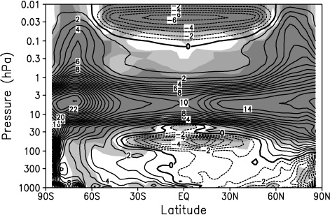
The response of the middle atmosphere to solar variability has been estimated from a variety of different datasets including lidar, rocketsonde, SSU/MSU, FUB as well as the NCEP and ERA-40 re-analyses. Here we present some of the results found by application of a multi-parameter regression analysis using the 11-year solar cycle (represented by the 10.7 cm flux) and a Quasi Biennial Oscillation (QBO) signature, all superposed on a trend which is assumed to be linear. Volcanic effects are dealt with either by inclusion of a stratospheric aerosol index or by removing data for the two years following major eruptions. Figure 1 shows the annual mean signal from rocketsonde data (1969-early 1990s) grouped into three latitude bands. Figure 2(a) presents the analysis of zonal mean SSU satellite data, as analysed by Nash (see Ramaswamy et al, 2001) and completed down into the Lower Stratosphere (LS) by MSU and Figure 2(b) the same from ERA-40. It is to be noted that in ERA-40, the TOVS, ATOVS and SSU instruments are used as radiances in the data assimilation. Up to about 10 hPa, radiosonde data is used in the data assimilation to bias correct all instruments but above this height, the model has no other reference. However for the recent period, AMSU-A channel 14 was used as reference to adjust SSU channels 2 and 3 with a fixed offset.

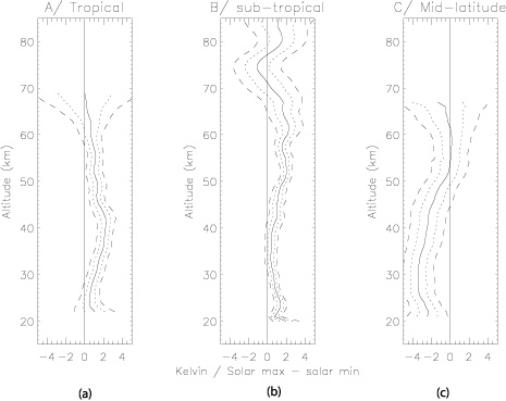
Figure 1. Annual mean temperature response (K) to solar activity (solar max – solar min). Responses from rocketsonde observations in: (a)Tropics (Ascension Island, 8°S; and Kwajalein, 9°N), (b) Northern subtropics (Barking Sands, 22°N; Cape Kennedy, 28°N; Point Mugu, 34°N) and (c) mid, high-latitudes (Shemya, 53°N; and Primrose Lake, 55°N). Dotted and dashed lines indicate 1 and 2 sigma error bars. The solar response is given for a full solar cycle having a mean amplitude of the solar forcing estimated from the last three cycles [from Keckhut et al., 2004].

(a)

(b)

Figure 2. (a) Zonal mean response from SSU/MSU data for the period 1979-1998, grey shading denotes statistical significance as shown in legend. (b) as (a) but from ERA-40 data for the period 1979-2001; light/dark shading denotes 95% and 99% significance (Crooks and Gray, 2004). Note the different height ranges in (a) and (b).

In all the datasets one can distinguish in the stratosphere three types of behaviour: the tropical region with a positive response of +1 to 2 K maximising just below the stratopause, a subtropical region indicating a much less significant response, but still positive, and a mid-latitude response which is negative. Seasonal analysis (not shown) reveals that the latter is determined by a large negative response in winter dominating a smaller positive summer signal.

There is more uncertainty in the vertical profile of the temperature response. In the tropical (25S-25N) LS a warming of 0.70 ± 0.18 K from minimum to maximum was found by Hood and Soukharev (2000) in MSU channel 4 data. The ERA-40 Re-analysis also shows a lower stratospheric signal maximizing near 20 to 30 degrees latitude in both hemispheres and near the 30 hPa level and a similar response is found in NCEP data (see Figures 7 and 11). The SSU and ERA-40 results, however, show significant disagreement with the latter presenting a local minimum at 10-20 hPa and the former suggesting a negative response around 50hPa. The reasons for these disagreements remain uncertain.

2.2. Observations of ozone

The amplitude of the solar signal in ozone has been investigated in observations from all available sources, namely: ground based (total column ozone, profile from Umkehr measurements), in situ measurements (ozonesonde profiles) and satellite observations.

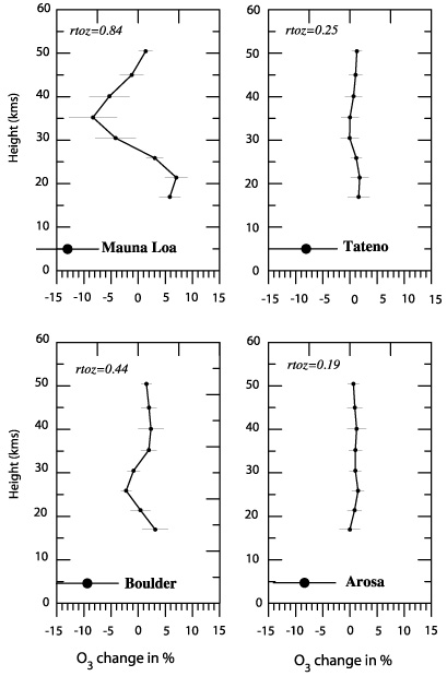
Sixteen stations measuring the vertical distribution of ozone with the Umkehr method were considered but quality checks suggested that only four Northern Hemisphere (NH) stations located between 19 and 47°N during the period 1957-2001 would qualify for the present analysis. These are Mauna Loa (20°N), Tateno (36°N), Boulder (40°N) and Arosa (47°N). Results are presented in Figure 3(a) for the period 1985-2002 (to make them comparable with the SAGE analysis) and generally show a positive response in the LS. Results from ozonesondes (not shown) are generally not statistically distinguishable from zero.

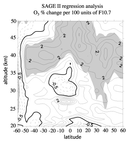
Ozone data in the form of ozone mixing ratio were derived from SAGE II (version 6.1) data, updated through June 2002 (end of the record), and used to construct 10° latitude belts from 60°S to 60°N. Even though the original data were retrieved from ground level up to the altitude of 70 km, the many missing data values and the volcanic aerosol data contamination force us to restrict the analysis to the range of altitudes from 20 – 50 km. Figure 3(b) shows higher ozone in the solar maximum phase, significant at altitudes from 35 – 45 km at all latitudes. Positive signals also extend to lower altitudes at mid-latitudes. This latter result is seen also in the ozonesonde as well as the Umkehr profile analysis at the stations of Arosa and Boulder, where the solar cycle signal becomes positive and significant at altitudes above about 20 km.
Although the largest percentage ozone changes over a solar cycle occur in the upper stratosphere, the corresponding column amounts are too small to explain the observed solar cycle variation of total ozone, which is several per cent, depending on latitude and season (Hood, 2004). Therefore, the observed lower stratospheric positive ozone response is likely to dominate the total ozone solar cycle variation at all latitudes. Solar cycle variation is the largest single form of long-term variability for ozone in the tropics and subtropics.

(a)	(b)
Figure 3. Annual mean ozone response to solar activity in units of percentage change per 100 F10.7 units (recent solar cycle amplitude ~130 F10.7 units). (a) Responses at four Umkehr stations for period 1957-2001, horizontal lines show 2-sigma range. (b) Zonal mean response from SAGE II data for the period October 1984-June 2002, contour interval 0.5 %, shading indicates regions of 95 % statistical significance.

2.3. Coupled chemistry-climate simulations

Model calculations have been performed with four models: two coupled chemistry-climate models by UKMO (UMETRAC see Austin and Butchart, 2003) and FUB (FUB-CMAM-CHEM see Pawson et al., 1998; Steil et al., 1998; Langematz, 2000), one chemical transport model by UIO (SCTM-1 see Rummukainen et al., 1999), and one 3D mechanistic model by CNRS (MSDOL developed by Service d'Aéronomie from the ROSE model).

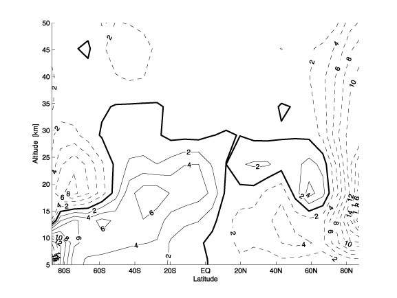
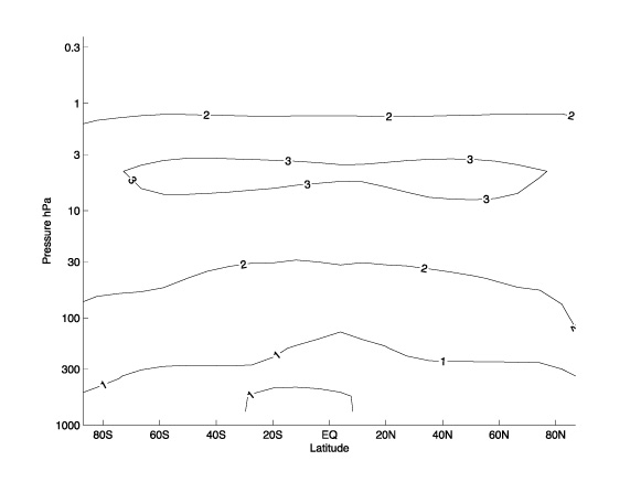
The relative importance of dynamics and photochemistry in determining the ozone response have been studied with SCTM-1. Figure 4(a) shows the results of changing the prescribed dynamical fields, according to the results of the Berlin GCM for the 11-year cycle response, without any changes in UV. This leads generally to an increase in ozone but with large decreases over the polar regions. Because of the large variability in high latitudes these changes are not statistically significant, but the tropical and sub-tropical increases in the LS are over 6%. The impact on ozone of solar UV changes alone peaks at just over 3% as shown in Figure 4(b), and are similar to the ozone changes previously calculated by 2D models (e.g. Haigh, 1994). The net effect of dynamical and chemical changes is dominated by the dynamical changes in the LS and also in the upper stratosphere at high latitudes.

(a)

(b)

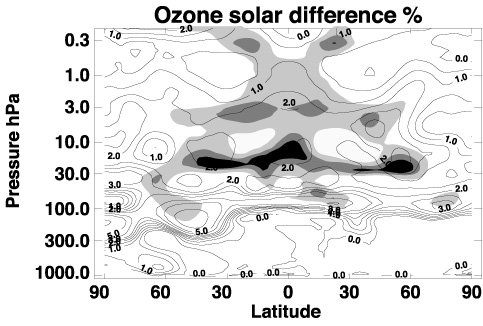
Figure 4. Annual mean, zonal mean, ozone response (%) to solar activity (solar max – solar min) in SCTM-1. (a) Due to imposing dynamical fields prescribed from the FUB-CMAM. (b) Due to changes in solar UV. The contour intervals are 2 % for (a) and 1 % for (b). Negative values are shown with dotted contours.

The coupled chemistry GCM ozone responses are shown in Figure 5 which shows the differences between steady state responses to solar maximum and solar minimum conditions (each run of several decades). UMETRAC and SCTM-1, like other previous investigations (see review by Shindell et al., 1999) compare poorly with observations, indicating insufficient ozone increase in the stratosphere and do not show the negative feature indicated in the observations in the LS (see above and Hood, 2004). In contrast, the FUB-CMAM-CHEM results compare favourably with observations in showing these two important features. It is likely, therefore, that some physical or chemical processes are missing from these other models that are present in FUB-CMAM-CHEM. The mesospheric ozone decrease in FUB-CMAM-CHEM results from enhanced catalytic destruction by HO_x, which is produced by enhanced Lyman-a irradiance during solar maximum. The shape and magnitude of the middle stratospheric ozone increase indicate an ozone response to the weaker thermospheric NO_x source in solar maximum, while the lower stratospheric ozone decrease is a combined effect of stronger chemical and dynamical ozone destruction in solar maximum (Langematz et al., 2004). This is due to an additional source of NO_x in the polar regions at the top of the model putatively due to Energetic Electron Precipitation (EEP), which is episodic but occurs more frequently during solar minimum. This decreases ozone during solar minimum above the mixing ratio peak and leads to a 'self healing effect' causing more ozone to be produced in the LS from the increased penetration of UV. Hence, the difference in ozone from solar minimum to solar maximum would be a larger increase in the upper stratosphere and a decrease in ozone in the LS relative to what would occur without the NO_x process included. This hypothesis has been put forward previously using 2-D models (Callis et al., 2001) but SOLICE is the first attempt to simulate these processes in a CCM. Several problems remain with regards to specifying the magnitude of the NO_x source and its transport from the upper mesosphere to the upper stratosphere. The FUB-CMAM-CHEM results suggest that it can be important, but further calculations need now to be made to confirm these findings.

(a)

(b)

Figure 5. Annual mean, zonal mean, ozone response (%) to solar activity (solar max – solar min) in (a) UMETRAC and (b) FUB-CMAM-CHEM. The shading denotes the regions of statistically significant change using a two-tailed t-test for the significance levels of 80 %, 95 % and 99 %.

Figure 6 shows the annual mean temperature change between solar minimum and maximum from the two CCM studies. The modelled impact generally increases with altitude from the LS to about 1 hPa. They are in reasonable agreement with observations in the middle and upper stratosphere, however, the models are not able to capture the secondary maximum in the observed temperature signal in the LS. The fields are somewhat noisy despite the long duration of the integrations, with the last 10 years (UMETRAC) or 14 years (FUB) analysed here. Part of this noise in UMETRAC is due to the presence of a QBO in the model; QBO effects are discussed further below. The lower stratospheric cooling shown by FUB-CMAM-CHEM is unique compared to other CCM simulations, and is due partially to changed chemical processes and partially due to less radiation coming from above (‘self healing effect’), as discussed above.

(a)

(b)

Figure 6. As Figure 5 but for temperature (K).

For the MSDOL simulations (CNRS, not shown) it was found that the level of lower-boundary wave-forcing in the model significantly affected the solar signal seen in the simulations. The use of climatologically averaged lower boundary forcing reduces the amount of wave forcing in the model. It was found that a preferential amplitude of forcing, equivalent to a magnification of 1.8 of the climatological value (assumed independent of solar variability), allowed maximum solar response. It was also found that, comparable to the solar signal in rocketsonde data, there was significant longitudinal variation in the solar response, particularly in the NH winter, emphasising the importance of zonal asymmetry in the solar response, and the fact that the longitudinal position must be taken into account when comparing observational data between themselves and with models (Hampson et al., 2004).

3. Interaction of the solar and QBO influences

3.1. Observations

Several publications (e.g., Labitzke, 1987, 2002; Labitzke and van Loon, 1988, 2000; van Loon and Labitzke, 2000) have shown that during the northern winters the signal of the solar cycle below 10 hPa emerges more clearly if the data are grouped according to the different phases of the QBO. This result was confirmed by Salby and Callaghan (2003) who defined for their study the northern winter period from September till February. It was shown further that during January/February, i.e. during the southern summers, the influence of the QBO is also large over the Southern Hemisphere (SH) (Labitzke, 2002). A summary of current ideas explaining the observed solar signal in the stratosphere is given in Kodera and Kuroda (2002), with emphasis on the dynamics over high latitudes during winter.

Here this work is extended to NH summer; during July and August the SH is relatively undisturbed by planetary wave activity and the solar signal can be found then relatively unobscured by dynamical interactions. The NCEP/NCAR re-analyses are used for the period 1968-2002. The data are grouped into years when the QBO in the LS (about 45 hPa) was in its west phase and years when it was in its east phase and our approach is to use a simple linear regression between temperature and 10.7 cm solar flux.

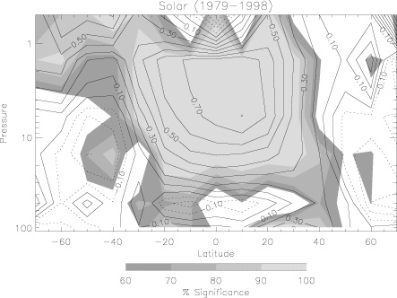
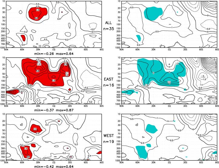
The vertical and meridional structure of the correlations between the solar cycle and the zonal mean temperatures from 1000 to 10 hPa is shown in Figure 7 for July together with the respective temperature differences between solar maxima and minima (taken to be 130 in 10.7 cm units). Over most of the Northern (summer) Hemisphere, extending to 30°S, the correlations (and temperature differences) are positive for the unsorted data. It is obvious, however, that the largest solar signal evolves for the data in the east phase of the QBO (middle panels). Here, the correlations above 0.5 cover a large height/latitude range. In the areas with large positive correlations/temperature differences one can assume adiabatic warm tropics and sub-tropics. The largest temperature difference, up to 2.5K are found at the 100-hPa level over the equator, that is around the tropical tropopause. Here, reduced stratospheric upwelling leads to a warming and lowering of the tropopause, e.g. Shepherd (2002). This hints to a connection to the meridional circulation systems (Hadley circulation in the troposphere and Brewer - Dobson circulation in the stratosphere) as suggested by Labitzke and van Loon (1995), Haigh (1996), Kodera and Kuroda (2002) and Salby and Callaghan (2003).

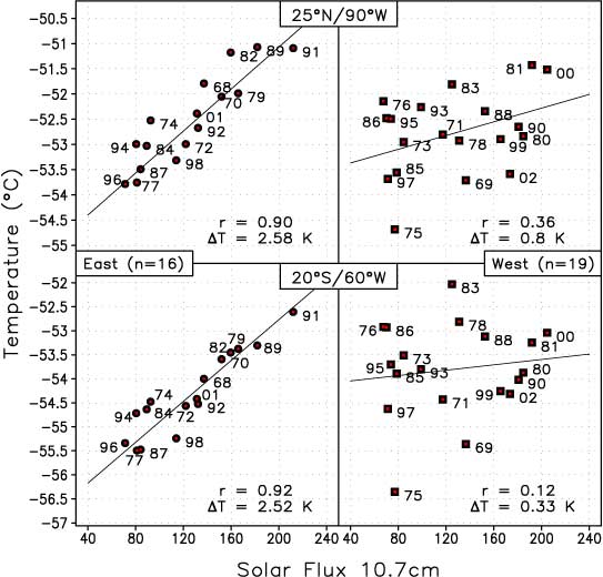
Figure 7. Left: Vertical-meridional sections of the correlations between the 10.7 cm solar flux and the de-trended zonal mean temperatures in July; shaded for emphasis where correlations are above 0.5. Right: The respective temperature differences (K) between solar maxima and minima, shaded where the correlations are above 0.5. Upper panels: all years; middle panels: only years in the east phase of the QBO; lower panels: only years in the west phase of the QBO. (NCEP/NCAR re-analyses, 1968-2002), (Labitzke, 2003).

The latitudinal distribution of the temperature and geopotential height solar signals has also been studied (not shown) and is found to be zonally fairly uniform. At 30 hPa in July warming is seen at all longitudes northward of 30°S with much stronger magnitudes during the QBO east phase. This is illustrated in Figure 8, which shows scatter plots of 30 hPa temperature against solar flux at two different locations (one in the summer and one in the winter hemisphere), in each case sorted into QBO east and west phases. In the east phase correlations exceed 90 % at both sites but in the west phase any relationship is very weak.

Figure 8. Scatter diagrams of de-trended 30-hPa temperatures (°C) against the 10.7 cm solar flux at two grid points. Upper panels: 25N/90W; lower panels:20S/60W. Left: years in the east phase of the QBO (n=16); right: years in the west phase (n=19). The numbers indicate the respective years; r=correlation coefficient, DT= temperature difference (K) between solar maxima and minima. Period: 1968-2002. (Labitzke 2003).

3.2. Mechanistic model studies

Direct solar heating of the atmosphere cannot explain the temperature response and its interaction with the QBO described in the previous section. A possible mechanism for the penetration of the solar signal, at least as far as the LS, is that the solar temperature response influences the zonal wind distribution (through thermal wind balance) and the altered wind distribution then influences the propagation of planetary waves through the stratosphere (Kodera and Kuroda, 2002; Hood, 2004).

Planetary wave forcing is known to be the precursor to Sudden Stratospheric Warmings (SSWs). Although SSWs are initiated at stratopause level, as they mature they extend vertically throughout the depth of the stratosphere and are, thus, an ideal vehicle for transferring a signal from the stratopause down into the lowest part of the stratosphere. Although the planetary wave propagation influence was proposed many years ago, the exact mechanism of this influence is still not understood very well. The influence mechanism is similar to that proposed for the QBO (Holton and Tan, 1980, 1982), in which the east phase of the QBO in the LS confines the planetary waves to high latitudes and, hence, they have greater impact on the polar vortex than during the west phase QBO. However, there is a conceptual problem with linking the mechanisms of influence, since the QBO is primarily a feature of the lower equatorial stratosphere, whereas the primary solar temperature response is in the upper equatorial stratosphere.

The UK Met Office Stratosphere Mesosphere Model (SMM) has been used to investigate the sensitivity of the modelled SSWs to zonal wind anomalies associated with the 11-year solar cycle and the QBO. Initial experiments (Gray et al., 2003) showed that increasing the planetary wave forcing resulted in earlier warmings and that when easterlies were imposed at the equator (at all heights) the warmings occurred earlier than when westerlies were imposed. In a second study (Gray, 2003), the SSWs were shown to be influenced by the winds in the LS, in agreement with the Holton-Tan mechanism, but they were even more sensitive to the imposed equatorial winds in the upper stratosphere. This is precisely the height region in which the solar influence is greatest, which suggests the possibility that the upper equatorial stratopause regions is where the solar and QBO influences interact. The observed amplitudes of the QBO and solar cycle wind anomalies at this level are also similar.

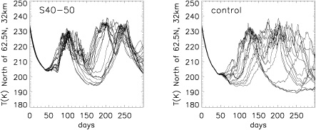
However, the wind anomalies associated with the 11-year solar cycle are not located directly over the equator but are found near the subtropical stratopause region. Further model experiments were carried out (Gray et al., 2004) in which an easterly anomaly (representing solar minimum conditions) was imposed in the subtropics between 40-50 km. It was imposed only for the first 60 days, to mimic an early winter anomaly. Figure 9 shows the evolution of north polar temperatures from this experiment. The 20 ensembles of the control run show considerable spread in the timing of the SSWs, with most of the warmings occurring around day 120. However, when the subtropical easterly anomaly is imposed, the timing of the warming shows much less variability and they occur at least 20 days earlier at day 100. The main result of these experiments is that the solar-induced wind anomaly in the subtropical upper stratosphere and the QBO-induced wind anomaly in the equatorial upper stratosphere can influence the timing of SSWs. The results suggest that under solar minimum conditions, with an easterly anomaly in the subtropical upper stratosphere, warmings are likely to occur earlier than in solar maximum conditions. Similarly, warmings are likely to occur earlier in QBO/E than in QBO/W years.

Figure 9. Ensemble of time-series of area-weighted, zonally-averaged modelled temperatures (K) north of 62.5°N, at 32 km from the subtropical easterly experiment (left) and the control experiment (right).

A proposed mechanism for the interaction of the solar signal and QBO has been suggested, based on these results (Gray et al., 2004). When the easterly anomalies associated with solar minimum and QBO/E reinforce each other, the warmings will speed up and occur in early-to-mid winter. When the westerly anomalies associated with solar maximum and QBO/W reinforce each other, the warmings will be slowed down but will, nevertheless, take place (unless they are slowed down so much as to prevent their occurrence before the end of winter). Thus, in both Smin/E years and Smax/W years there will be a clear solar/QBO signal. However, in the other combinations Smin/W and Smax/E the anomalies will partially cancel and, hence, there is less likely to be a clear solar/QBO signal in SSWs. This may help to understand the puzzling observation that SSWs occur in Smax/W years even though the QBO/W phase means that there is no waveguide in the LS in those years.

The modulation of the timing of SSWs by the 11-year solar cycle and the QBO will also modulate the strength of the meridional circulation. This, in turn, will modulate the strength of up-welling in the equatorial LS. This may help to explain the observed solar temperature response in the subtropical LS in Figure 2a in both summer and winter hemispheres since it will modulate the speed at which the QBO descends through this region of the atmosphere. The meridional pattern of the two subtropical lower stratospheric signals looks remarkably like the QBO temperature response. It may also explain other observations (e.g. Salby and Callaghan, 2000) which show a solar modulation of the length of the westerly QBO phase.

3.3. GCM simulations

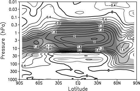
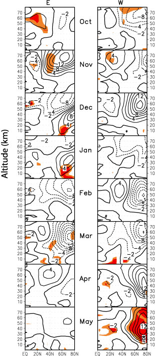
In the long-term mean state many GCMs, including FUB-CMAM, are not able to reproduce a realistic QBO (e.g., Pawson et al., 2000), so to simulate its effect zonal wind anomalies are prescribed over the equator. Solar experiments with prescribed solar UV and ozone changes were carried out in the FUB-CMAM with artificially imposed QBO westerlies only in the LS. These experiments failed to reproduce the observed relationship between the solar and the QBO signals. Therefore, further experiments were performed in which rocketsonde data from Gray et al. (2001) were used to impose a QBO signal not only in the LS but also in the upper stratosphere. These model experiments with the FUB-CMAM have confirmed for the first time with a GCM the results of recent observational and Rutherford Appleton Laboratory (RAL) mechanistic model studies discussed above (Matthes et al., 2004). By imposing more realistic equatorial winds throughout the stratosphere, the model produces an improved simulation of the polar night jet (PNJ) and mean meridional circulation (MMC) response to solar cycle variations. The model results are now in good agreement with observational data (Kodera and Kuroda, 2002; Hood, 2004). Figure 10 shows the poleward downward movement of the mean zonal mean wind differences between solar maximum and minimum for QBO easterlies (Figure 10a) and QBO westerlies (Figure 10b) which was not produced previously (Matthes et al., 2003).

Figure 10. FUB-CMAM results, long-term mean wind differences between solar maxima and minima for the QBO east (left) and the QBO west experiments (right) for the NH from October to May and from the surface to 80 km (1000 to 0.01 hPa), contour intervals 2 m/s. Light (heavy) shading indicates the 95 % (99 %) significance level (Student t-test). Similar to Fig. 13a,b from Matthes et al., 2004.

The results indicate that the QBO determines the timing, rather than the existence, of the solar signal. Stratospheric warmings during the westerly phase of the QBO and during solar maximum years occur already in January, whereas they appear one month later for the easterly phase. The Holton and Tan relationship is evident during solar minimum years, whereas it is less clear for the solar maximum experiments in agreement with observations.

Experiments with the Met Office Unified model (not shown) also confirm that equatorial stratospheric wind anomalies associated with the QBO and solar cycle can interact to influence the development of the wintertime circulation at higher latitudes (Palmer and Gray, 2004).

4. Solar influence in the troposphere

4.1. Observations

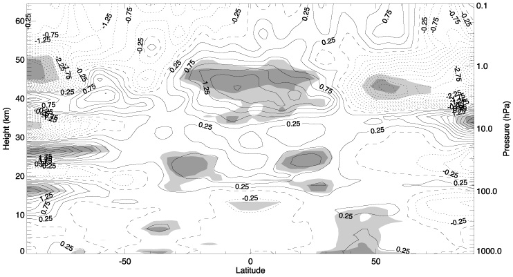
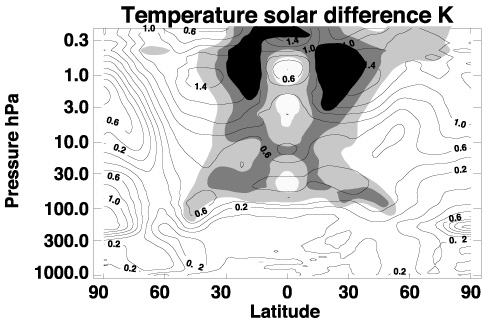
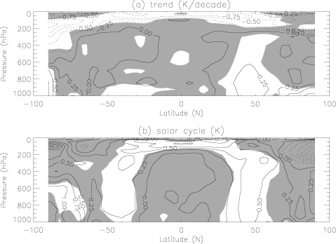
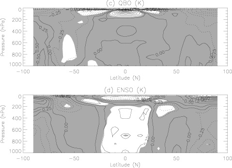
A multiple regression analysis of zonal mean temperature data from the NCEP/NCAR reanalysis dataset (using data from 1979 only as the lower stratospheric data are suspect before that date) has been carried out (Haigh, 2003). The analysis incorporated an autoregressive noise model of order one and eleven indices: a constant, a linear trend, the solar 10.7cm flux, the QBO, the El Niño-Southern Oscillation, stratospheric aerosol loading (related to volcanic eruptions), North Atlantic Oscillation (NAO) and four indices representing the amplitude and phase of the annual and semi-annual cycles. Figure 11a shows a strong cooling trend in the stratosphere and warming in the troposphere in mid-latitudes. The solar signal is presented in Figure 11b with warming in the tropical LS at higher levels of solar activity extending in vertical bands into the troposphere in both hemispheres at latitudes 20°-60°. It is interesting to note that, while the stratospheric signal is similar to that shown by Labitzke (2003) using a single parameter regression on de-trended data (see Figure 6) the tropospheric pattern is not the same and the solar response in the troposphere is generally deduced to be larger when the other factors (QBO, ENSO etc) are taken into account in a multiple regression. Care has to be taken when comparing Figure 6, which is for July, with Figure 10, representing an annual mean but both results are broadly consistent with the solar signal of ~0.4 K shown in the NH upper troposphere temperatures in July and August by van Loon and Shea (1999). The effects of the QBO (Figure 11c) are largely confined to the tropical LS while the ENSO signal (Figure 11d) is seen clearly throughout the tropics. Volcanic eruptions cause the stratosphere to warm and the troposphere to cool (Figure 11e), while the NAO signal (Figure 11f) is mainly confined to NH mid-latitudes.

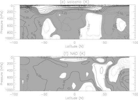
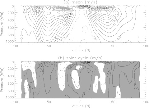
Figure 11. Amplitudes of the components of variability in NCEP (1979-2000) zonal mean temperature due to: (a) trend (b) solar, (c) QBO, (d) ENSO, (e) volcanoes, (f) NAO. The units are K/decade for the trend, otherwise maximum variation (K) over the data period. Shaded areas are not statistically significant at the 95 % level using a Student’s t test. Haigh, 2003.

A similar multiple regression analysis of zonal mean zonal wind data from the NCEP/NCAR re-analysis has been carried out; some of the results are shown in Figure 12. These observations show that the sub-tropical jets are weaker and further poleward at solar maximum than at solar minimum. It is worth noting that the hemispheric symmetry in the solar plot provides further support for the robustness of the signal (the values at each point being derived independently) and that the solar and NAO signals are independent. If the sun is influencing the NAO, then some of the NAO signal in Figures 10,11 may be ascribed to the sun – but not vice versa.

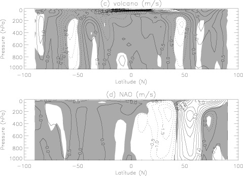
Figure 12. (a) Annual mean, zonal mean, zonal wind (m/s) from NCEP (1979-2002); (b) amplitude of the solar component; (c) volcanic component; (d) NAO. Shaded areas are not statistically significant at the 90% level using a Student’s t test. Haigh et al., 2004.

4.2. Simplified GCM experiments

Experiments with full GCMs (Haigh, 1996, 1999; Larkin et al., 2000; FUB-CMAM, this project) have suggested that the response in the troposphere is a weakening and poleward shift of the sub-tropical jets and a weakening and expansion of the Hadley cells at solar maximum relative to solar minimum. This pattern is remarkably similar to that resulting from the multiple regression study of zonal winds presented in section 4.1 and of vertical velocities by Gleisner and Thejll (2003). These models all used fixed sea surface temperatures so the influence must be induced by the direct solar effects in the stratosphere.

The simplest explanation for this behaviour is that the increase in static stability induced by the stratospheric heating reduces vertical velocities in the tropics and, thus, weakens the Hadley circulations. This is a plausible first step but does not explain the Hadley cell expansions nor the jet stream shifts.

The direct solar heating of the tropical lower stratospheric may be enhanced by changes in the mean circulation of the middle atmosphere induced by modulation of planetary wave propagation, as discussed in section 2, and it seems clear that these effects are important in determining the QBO/solar interaction. However, the GCM used in the original demonstration of the impact of solar UV variability on the troposphere (Haigh, 1996) only extended to 10 hPa and the Larkin et al. (2000) model, which showed the effects on tropospheric winds and circulation throughout the year, extended only to 0.1 hPa so it appears that, at least for the tropospheric effects discussed in section 4.1, a full simulation of the middle atmosphere is not necessary.

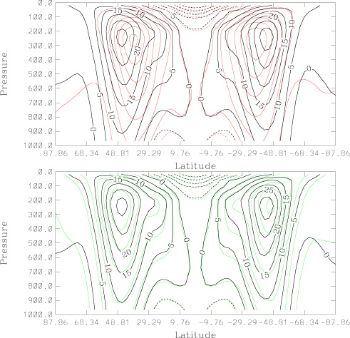
In order to understand the mechanisms underlying the observed tropospheric variability associated with solar and volcanic forcing, we have performed some idealised-forcing experiments using a simplified Global Circulation Model (sGCM) (Haigh et al., 2004), which includes full dynamics but temperature is relaxed towards a zonally symmetric equilibrium distribution. Experiments with the model have been designed to investigate the effects of perturbations to the temperature structure of the LS by varying the values used for the radiative equilibrium temperatures in the LS. Experiment U5 prescribes a uniform increase of 5 K throughout the stratosphere, while in experiment E5 the equatorial stratosphere is warmed by 5 K but this is gradually reduced to zero increase at the poles. The zonal mean zonal wind field found in the two sGCM experiments are presented in Figure 13, each overlaid on the control field. Run U5 shows a weakening of the jet and a large equatorward shift, while the response of experiment E5 is a weakening and latitudinal expansion, but mainly poleward shift, of the jets. The patterns are, thus, qualitatively similar to the volcanic and solar signals, respectively, found in the multiple regression analysis of NCEP data (Figure 11).

Figure 13. Zonal mean, zonal winds from simple GCM experiments; control run in black with (a) experiment U5 overlaid in red and (b) experiment E5 overlaid in green. Negative contours are dashed, contour interval is 5 ms-1. Haigh et al., 2004

The experiments with the sGCM provide some indications as to how these responses arise. All runs (including several not shown) in which thermal perturbations were applied only in the LS show effects throughout the troposphere, with the vertically banded anomalies in temperature and zonal wind typical of the results of the data analysis, and changes in the tropospheric mean circulation. Heating the LS increases the static stability in this region, lowers the tropopause and reduces the wave fluxes here. This leads to coherent changes through the depth of the troposphere, involving the location and width of the jetstream, storm-track and eddy-induced meridional circulation.

The precise shape of the patterns of response depends on the distribution of the stratospheric heating perturbation: heating at mid- to high latitudes causes the jets to move equatorwards and the Hadley cells to shrink, while heating only at low latitudes results in a poleward shift of the jets and an expansion of the Hadley cells. We, therefore, suggest that the observed climate response to solar variability is brought about by a dynamical response in the troposphere to heating predominantly in the stratosphere. The effect is small, and frequently masked by other factors, but not negligible in the context of the detection and attribution of climate change. The results, of both the sGCMs and full GCMs, also suggest that at the Earth’s surface the climatic effects of solar variability will be most easily detected in the sub-tropics and mid-latitudes.

5. References

Austin, J. and N. Butchart, Coupled chemistry-climate model simulations for the period 1980 to 2020: Ozone depletion and the start of ozone recovery, Q.J. Roy. Meteorol. Soc., 129, 3225-3249, 2003.

Callis, L.B., et al., Solar-atmosphere coupling by electrons (SOLACE), 3, Comparisons of simulations and observations, 1979-1997, issues and implications, J. Geophys. Res., 106, 7523-7539, 2001.

Gleisner, H. and P. Thejll, Patterns of tropospheric response to solar variability. Geophys.Res.Lett., 30, 1711, doi:10.1029/2003GL017129, 2003.

Gray, L.J., The Influence of the equatorial upper stratosphere on stratospheric sudden warmings. Geophys. Res. Letts. 30(4) doi: 10.1029/2002GL016430, 2003.

Gray, L.J., et al., Solar and QBO influences on the timing of stratospheric warmings. J. Atmos. Sci., submitted, 2004.

Gray, L.J., et al., On the interannual variability of the Northern Hemisphere stratospheric winter circulation: The role of the QBO. Quart. J. Roy. Meteorol. Soc. 127, 1413-1432, 2001.

Gray, L.J., et al., The influence of the equatorial upper stratosphere on Northern Hemisphere stratospheric sudden warmings. Quart. J. Roy. Meteorol. Soc. 127, 1985-2003, 2003.

Haigh, J.D., The role of stratospheric ozone in modulating the solar radiative forcing of climate, Nature, 370, 544-546, 1994.

Haigh, J.D., The impact of solar variability on climate. Science, 272, 981-984, 1996.

Haigh, J.D., A GCM study of climate change in response to the 11-year solar cycle. Quart.J. Roy.Meteorol.Soc., 125, 871-892, 1999.

Haigh, J.D., The effects of solar variability on the Earth’s climate. Phil. Trans. Roy. Soc. 361, 95-111, 2003.

Haigh, J.D., et al., The response of tropospheric circulation to perturbations in lower stratospheric temperature. Submitted to J. Clim, 2004.

Hampson, J., et al., The 11-year Solar-Cycle Effects on the Temperature in the Upper-Stratosphere and Mesosphere: Part II Numerical Simulations and the Role of Planetary Waves. Submitted to J. Atmos. Sol.-Terrest. Phys., 2004.

Holton, J.R. and H.C. Tan, The influence of the equatorial quasi-biennial oscillation on the global circulation at 50 mb., J. Atmos. Sci., 37, 2200-2208, 1980.

Holton, J.R. and H.C. Tan, The quasi-biennial oscillation in the Northern Hemisphere lower stratosphere, J. Meteor. Soc. Jpn., 60, 140-148, 1982.

Hood, L.L., Effects of solar UV variability on the stratosphere, In “Solar variability and its effect on the Earth’s atmosphere and climate system”, AGU Monograph Series, Eds. J. Pap et al., American Geophysical Union, Washington D.C., in press, 2004.

Hood, L.L. and B.E. Soukharev, The solar component of long-term stratospheric variability : observations, model comparisons, and possible mechanisms. Proc. 2nd SPARC General Assembly, Mar del Plata, Argentina, 2000.

Keckhut P, et al., The 11-year Solar-Cycle Effects on the Temperature in the Upper-Stratosphere and Mesosphere: Part I Assessments of observations. Submitted to J. Atmos. Sol.-Terrest. Phys., 2004.

Kodera, K., and Y. Kuroda, Dynamical response to the solar cycle, J. Geophys. Res., 107, 4749, 2002.

Labitzke, K., Sunspots, the QBO, and the stratospheric temperature in the north polar region. Geophys. Res. Lett., 14, 535-537, 1987.

Labitzke, K., The Solar Signal of the 11-year sunspot cycle in the stratosphere: Differences between the Northern and Southern summers, J. Meteorol. Soc. Japan. 80, 963-971, 2002.

Labitzke, K. and H. van Loon, Associations between the 11-year solar cycle, the QBO and the atmosphere. Part I: The troposphere and stratosphere in the Northern Hemisphere winter. J.A.T.P., 50, 197-206, 1988.

Labitzke, K. and H. van Loon, Connection between the troposphere and the stratosphere on a decadal scale. Tellus, 47 A, 275-286, 1995.

Labitzke, K. and H. van Loon, The QBO effect on the global stratosphere in northern winter. J.A.S.-T.P., 62, 621-628, 2000.

Langematz, U., An estimate of the impact of observed ozone losses on stratospheric temperature. Geophys. Res. Lett., 27, 2077-2080, 2000.

Langematz, U., et al., Chemical effects in 11-year solar cycle simulations with the Freie Universität Berlin Climate Middle Atmosphere Model with online chemistry (FUB-CMAM-CHEM), in preparation, 2004.

Larkin A., et al., The effect of solar UV irradiance variations on the Earth’s atmosphere. Space Sci.Rev., 94, 199-214, 2000.

Matthes, K., et al., GRIPS solar experiments intercomparison project: initial results, Meteorology and Geophysics. 54, 71-90, 2003.

Matthes, K., et al., Improved 11-Year Solar Signal in the Freie Universität Berlin Climate Middle Atmosphere Model. J. Geophys. Res. doi:10.1029/2003JD004012, 2004.

Palmer, M.A. and L.J. Gray, Modelling the response to solar forcing with a realistic QBO. In preparation, 2004.

Pawson, S., et al., The GCM-Reality Intercomparison Project for SPARC (GRIPS): Scientific issues and initial results, Bull. Am. Meteorol. Soc., 81, 781-796, 2000.

Pawson, S., et al., The Berlin troposphere-stratosphere-mesosphere GCM: Sensitivity to physical parametrizations, Q. J. R., Meteorol. Soc., 124, 1343-1371, 1998.

Ramaswamy, V., et al., Stratospheric temperature trends: observations and model simulations, Rev. Geophys., 39, 71-122, 2001.

Rummukainen, M., et al., A global model tool for three-dimensional multiyear stratospheric chemistry simulations: Model description and first results. J. Geophys. Res., 104, 26437-26456, 1999.

Salby, M. and P. Callaghan, Connection between the solar cycle and the QBO: The missing link. J. Clim., 13, 2652—2662, 2000.

Salby, M. and P. Callaghan, Evidence of the solar cycle in the general circulation of the stratosphere. J. Clim., 17, 34-46, 2004.

Shepherd, T.G., Issues in stratosphere-troposphere coupling. J. Met. Soc. Japan, 80, 769-792, 2002.

Shindell, D., et al., Solar cycle variability, ozone and climate, Science, 284, 305-308, 1999.

Steil B, et al., Development of a chemistry module for GCMs: first results of a multiannual integration. Annal.Geophys. 16, 205-228, 1998.

Van Loon, H. and K. Labitzke, The Influence of the 11-Year Solar Cycle on the Stratosphere Below 30km: a Review. Space Sci. Rev. 94, 259-278, 2000.

Van Loon, H. and D. Shea, A probable signal of the 11-year solar cycle in the troposphere of the Northern Hemisphere. Geophys.Res.Lett., 26, 2893-2896, 1999.