S P A R C Stratospheric Processes And their Role in Climate A project of the World Climate Research Programme Home Initiatives Organisation Publications Meetings Acronyms and Abbreviations Useful Links

Major stratospheric warming in the Southern Hemisphere in 2002: Dynamical aspects of the ozone hole split

Mark Baldwin, Northwest Research Associates, Bellevue, USA (mark@nwra.com)
Toshihiko Hirooka, Kyushu University, Fukuoka, Japan (hirook@geo.kyushu-u.ac.jp)
Alan O'Neill, University of Reading, Reading, UK (alan@met.reading.ac.uk)
Shigeo Yoden, Kyoto University, Kyoto, Japan (yoden@kugi.kyoto-u.ac.jp)
and collaborators*

Collaborators*: A.J. Charlton (Univ. of Reading), Y. Hio (Kyoto Univ.), W.A. Lahoz (Univ. of Reading), and A. Mori (Kyushu Univ.).

Introduction

In late September 2002 the Southern Hemisphere stratosphere underwent its first recorded major stratospheric warming, splitting the vortex and tearing the normally quiescent Antarctic ozone hole into two parts. The occurrence of this “unprecedented event” (WMO, 2002), in which the stratosphere suddenly warmed, is in contrast to the trend for the last ~20 years toward a stronger, colder, longer-lasting Antarctic vortex. Why did a major warming occur in the Southern Hemisphere? Was its occurrence somehow related to ozone or climate trends, or was it simply a highly unusual event? What are the implications for future ozone and climate trends?

Several weeks after the event, in November 12–15, the “International Symposium on Stratospheric Variations and Climate” was held at Kyushu University, Fukuoka, Japan (Miyahara et al., 2003, this issue). Following the suggestion by J.R. Holton, we had a special discussion session on the sudden warming and split of the Antarctic ozone hole. Preliminary results on several dynamical aspects were presented by the authors, followed by an intensive discussion session.

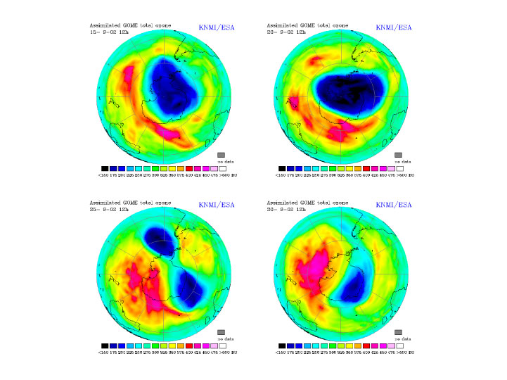
Figure 1 shows time evolutions of the total ozone field assimilated at KNMI (the Royal Netherlands Meteorological Institute). Animations on the special events, which are also available at their WEB site (http://www.knmi.nl/gome_fd/index.html), clearly show that the elongated ozone hole rotated eastward in mid September, and shifted off the pole just before the event. The highly elongated ozone hole split into two parts, with the smaller part equatorward of the northwest side of the Antarctic Peninsula disappearing by the end of September.

Figure 1. Time evolution of the total ozone field assimilated at KNMI: September 15, 20, 25, and 30 in 2002. http://www.knmi.nl/gome_fd/index.html

Time evolution of the polar vortex

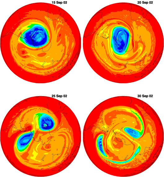
The dramatic split and subsequent breakdown of the polar vortex, as well as the accompanying mixing of high-and low-latitude stratospheric air are clearly shown by the sequence of high-resolution fields of Ertel's potential vorticity (PV) of Figure 2. On 15 September, the vortex is characterised by high (modulus) values of PV (indicated in blue), with a sharp gradient of PV in the associated strong westerly jet stream. Outside the vortex at mid latitudes, gradients of PV are small as a result of the mixing of PV by transient, large-scale anticylones in the stratosphere, which track eastwards around the polar vortex. Such a flow regime is characteristic of the stratosphere in the Southern Hemisphere at this time of year, and is often accompanied by an elongated polar vortex (Mechoso et al., 1988).
Figure 2 shows such an elongated polar vortex on 20 September, a few days prior to the split. It seems plausible to regard the elongated vortex as being in a preconditioned state to split (e.g. by tropospheric effects or dynamical instability). The subsequent split leads, on 25 September, to two distinct centres of high (modulus) PV connected by a long thin streamer of air from the edge of the polar vortex. A large anticylone, centred between Antarctica and Australia, and a weaker anticylone over the South Atlantic, is evidenced by weak gradients of PV in these regions. Once the vortex has split, the individual vortices are rapidly weakened by the shearing out of PV around the anticyclones, as indicated on 30 September.

Figure 2. Potential vorticity on the 850K isentropic surface (near 10 hPa) for the Southern Hemisphere on the dates shown during September 2002. The fields are derived from high-resolution (T511) meteorological analyses provided by the European Centre for Medium Range Weather Forecasts. On each chart, the Greenwich Meridian is at the top. Values of potential vorticity associated with the stratospheric polar vortex are indicated with the colour blue.

Evolution of the SH polar vortex during the past 24 years

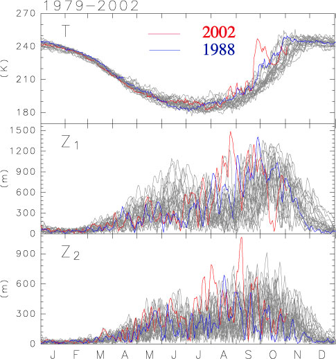
Figure 3 shows the daily evolution of two quantities which characterise the polar vortex from 1979 to 2002: temperature at the South Pole (top) and geopotential height amplitudes of zonal wavenumber 1 (middle) and 2 (bottom) in high latitudes, at the 20 hPa level. The polar temperature in late September 2002 was extremely high (red line), indicating this is an unprecedented event at least in the past 24 years. Three minor warming events are also observed in late August and early to mid September, which are comparable to that in 1988 (blue line). These warming events are associated with amplification of planetary waves. The daily amplitude of wavenumber 1 is very large in August 2002, while that of wavenumber 2 is large in July and early September. We note that the largest amplitudes of wave 1 and wave 2 ever observed occurred during the winter of 2002.

Figure 3. 24-year records of the daily evolution of the polar vortex (NCEP/NCAR reanalysis from 1979 to 2002): temperature at the South Pole (T), geopotential-height amplitudes of zonal wavenumber 1 (Z1) and 2 (Z2) averaged over the latitudes between 60°S and 70°S, at the 20 hPa level.

Year-to-year variations of the monthly mean of the daily amplitudes of zonal wavenumber 1 and 2 are shown in Figure 4 for July (a), August (b), September (c), and October (d), together with the monthly temperature at the pole in colour. The monthly mean values for both wavenumbers are large in July, August and September 2002, although either amplitude in some years is comparable to that in 2002 (e.g., [Z1] in 1988 and [Z2] in 1997 in September). The planetary waves in the polar region are quite active through the winter 2002.

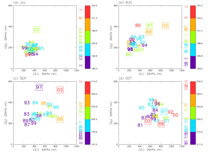
Figure 4. 24-year records of the monthly mean of daily geopotential-height amplitudes of zonal wavenumber 1 [Z1] and 2 [Z2] averaged over the latitudes between 60°S and 70°S, at the 20 hPa level. Monthly mean temperature at the pole is also shown with colour indicated on the right side of each panel.

Vertical linkage of the events

Here we describe the vertical linkage of the events on the basis of the U.K. Met Office stratospheric assimilated data and compare it with a typical year (2001) when the usual seasonal march was observed. Figure 5 shows time-height sections of the zonal mean zonal wind at 60°S for the period from July to October in 2002 (top) and 2001 (bottom). In 2002, we can see a regularly oscillatory change of the polar night jet with a typical time scale of about 10 days throughout the winter season prior to the sudden warming. Eventually, the sudden warming occurred on 26 September, with winds reversing to easterly at 10 hPa, 60°S and a reversal of the temperature gradient between 60°S and the pole, meeting the WMO criteria for a major stratospheric warming.

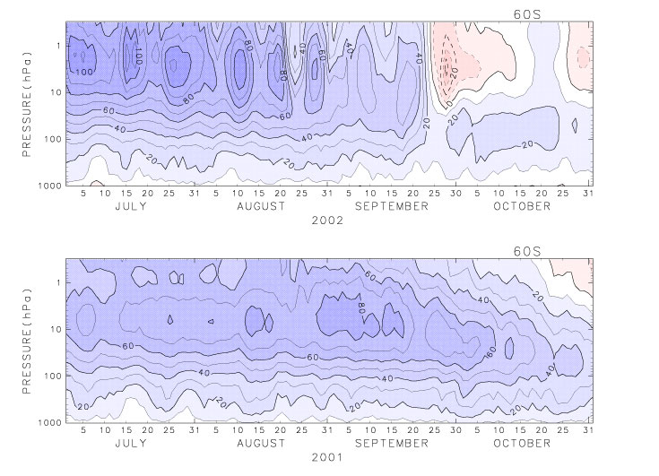
Figure 5. Time-height sections of the zonal mean zonal wind at 60°S for the period from July to October in 2002 (upper panel) and 2001 (lower panel). Units are ms-1 and the contour interval is 10 ms-1. Blue shading denotes the westerlies while red denotes the easterlies.

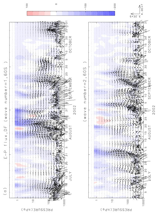
Figure 6 illustrates time-height sections of the Eliassen-Palm flux at 60°S and the wave driving due to its divergence of zonal wavenumbers 1 and 2 for the period from July to October in 2002 and 2001. From these panels, it can be seen that planetary wave activities of both wavenumber 1 and 2 are very strong throughout the period in 2002 while those are relatively weak in 2001. These periodic strengthening seen in 2002 corresponds to the regular oscillation of the polar night jet. In particular, the difference between the two years is fairly large in the upper stratosphere due to the frequent occurrence of vertical propagation of planetary waves, which results in the strong deceleration of the westerlies. However, the deceleration giving rise to the sudden warming is rather inconspicuous, whereas the strong deceleration can be seen in the second half of August. As shown in Figure 5, such strong deceleration corresponds to the sequential occurrence of minor warmings; after that the strong polar vortex could not be fully re-established. Hence, it appears that the vortex was fairly vulnerable to planetary-wave activity, i.e., preconditioned. The conditions necessary for the major warming were in fact the results of several minor warming events during mid-to-late winter.

Figure 6. Time-height sections of the Eliassen-Palm (E-P) flux (vectors) at 60°S and the wave driving (shading) due to its divergence for the period from July to October in (a) 2002 and (b) 2001. Each upper panel shows the contribution of zonal wavenumber 1 and lower shows that of zonal wavenumber 2. The arrow scale denotes vertical and horizontal components of the E-P flux vector (kgs-2) and the right direction corresponds to the poleward. Blue shading denotes zonal wind deceleration while red denotes acceleration; see the tone bar where the units are ms-1day-1.

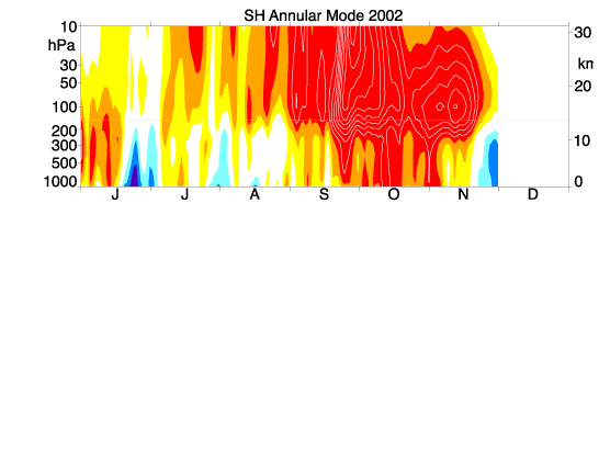
Southern Annular Mode

The warming event was remarkable not just for its intensity, but for its duration, penetration to the lowermost stratosphere, and coupling to the surface. The time-height development of the event can be seen through changes in the Southern Annular Mode (SAM) (Figure 7). The SAM patterns are a measure of the strength of the polar vortex at each pressure level, and are defined as the leading empirical orthogonal function of slowly varying (in this case 90-day low-pass filtered) geopotential anomalies. At each level a positive SAM (blue) corresponds to a strong vortex, with negative geopotential anomalies ove r the polar cap and positive geopotential anomalies over midlatitudes (Thompson and Wallace, 2000).
In Figure 7 the stratospheric vortex was weaker than normal throughout the winter, with 10-hPa values continuously negative until the end of November. The major warming was preceded by nearly three months of an anomalously weak stratospheric vortex, becoming much weaker during September (the average stratospheric SAM value in September before the onset of the warming is ~ –2s).
The troposphere was not unusual before September, but during September the tropospheric SAM also became negative, and remained continuously negative during September, October, and most of November. This is consistent with behaviour seen in the Northern Hemisphere in which the tropospheric NAM tends to be biased toward the NAM in the lowermost stratosphere near 150 hPa (Baldwin and Dunkerton, 2001). The long time scale of the tropospheric SAM is also consistent with the long-lived stratospheric anomaly. What is not obvious in Figure 7 is a clear downward propagation of stratospheric anomalies, as seen in Baldwin and Dunkerton (2001). In terms of the SAM, the warming appears to have occurred first in the lowermost stratosphere, rather than propagating downward. However, the most negative SAM values, exceeding –6s, occurred at 10 hPa, coincident with the warming.
The warming event was not only unprecedented in the Southern Hemisphere, but the SAM values exceeded those seen in the Northern Hemisphere. An event of this magnitude, intensity, and duration has never been observed in either hemisphere.

Figure 7. Time-height development of the SAM during 2002. The daily SAM index for each level is obtained by projecting daily geopotential anomalies onto the SAM patterns. Blue corresponds to positive values (strong, cold vortex), while red corresponds to negative values (warm, weak vortex). The values at each level are normalised by the standard deviation of the September-November index during 1979-2001. The contour interval is 0.5s, with values between –0.5s and 0.5s unshaded. The thin horizontal line is at 150 hPa.

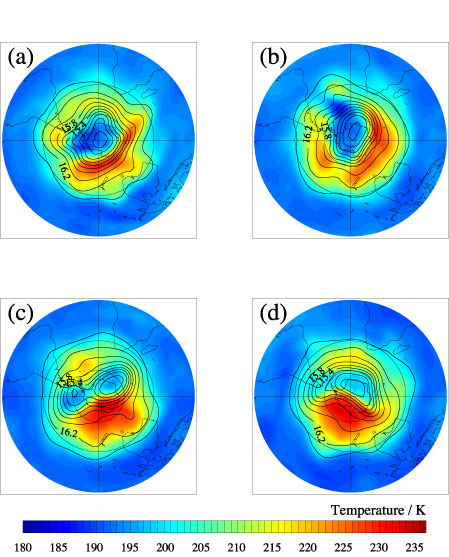
Upper troposphere and lower stratosphere

Figure 8 shows a sequence of fields of geopotential height and temperature at 100 hPa near the base of the stratosphere during the time of the split. The circulation is dominated by a strong westerly vortex (a), with a zonally asymmetric temperature structure. The strongest temperature anomaly is located between Antarctica and Australia, overlying the stronger of the two anticyclones involved in splitting the stratospheric polar vortex. The westerly vortex at 100 hPa evolves into two distinct cyclonic centres (c) in unison with the split in the stratospheric polar vortex, recombining into one centre (d) as the stratospheric polar vortex breaks down. Modelling studies will be needed to determine whether this evolution of the vortex in the upper troposphere and lower stratosphere near 100 hPa can be regarded as having "forced" the split of the stratospheric polar vortex.

Figure 8. Fields of geopotential height (contours at intervals of 0.2 km) and temperature (colours given by the scale at the bottom of the figure) at 100 hPa for the Southern Hemisphere (a) 15, (b) 20, (c) 25 and (d) 30 September 2002. The fields are derived from meteorological analyses provide by the U.K. Met Office. On each chart, the Greenwich Meridian is at the top.

Concluding remarks

In order to discuss the rarity of the stratospheric sudden warming event in September in the Southern Hemisphere, we refer to a recent work by Taguchi and Yoden (2002) with a simple global circulation model. They investigated interannual variations of the troposphere-stratosphere coupled system based on 1,000 year integrations. In a run corresponding to the Southern Hemisphere, a highly skewed distribution of the polar temperature in the upper stratosphere is obtained for the months from April to September (their Figures 1 and 2). The probability distribution is far from the normal (Gaussian) distribution, and about 0.5 % of the 1,000 years are extremely warm with a monthly temperature anomalies exceeding 6s. The skewed probability distribution requires careful treatment in the statistical arguments of the rarity. The possibility of major warmings in the Southern Hemisphere is also supported by some GCM experiments - prior to September 2002 the occasional major warmings in the Southern Hemisphere were considered a model “defect.”

We are not aware of any results that implicate climate or ozone trends in the occurrence of the 2002 major warming, and we find no evidence that this event should change our expectations concerning the recovery of the ozone hole over the next few decades. Rather, it appears that the event was simply unusual - perhaps a one in fifty or one hundred year event. However, despite carefully worded press releases and scientific papers, it is difficult to avoid the public perception that natural processes “filled in” the 2002 ozone hole and that the ozone hole will be less of a problem in the future.

References

Baldwin, M.P., and T.J. Dunkerton, 2001, Stratospheric harbingers of anomalous weather regimes, Science, 294, 581-584.
KNMI: GOME Assimilated Ozone Fields is available at GOME FAST DELIVERY SERVICE. http://www.knmi.nl/gome_fd/index.html

Mechoso, C.R., et al., 1988, A study of the stratospheric final warming of 1982 in the Southern Hemisphere. Quart. J. Roy. Meteorol. Soc., 114, 1365-1384

Miyahara, S., et al., 2003, Report on the International Symposium on “Stratospheric Variations and Climate”, SPARC Newsletter, this issue.

Taguchi, M., and S. Yoden, 2002, Internal interannual variations of the troposphere- stratosphere coupled system in a simple global circulation model. Part II: Millennium integrations. J. Atmos. Sci., 59, 3037-3050.

Thompson, D.W.J., and J.M. Wallace, 2000, Annular modes in the extratropical circulation. Part 1: Month-to-month variability, J. Climate, 13, 1000-1016.

WMO, 2002, Antarctic ozone hole splits in two. Press Release No. 681, 1 October, 2002.