 |
Stratospheric Processes And their Role in Climate
|
||||||||
| Home | Initiatives | Organisation | Publications | Meetings | Acronyms and Abbreviations | Useful Links |
![]()
|
Stratospheric Processes And their Role in Climate
|
||||||||
| Home | Initiatives | Organisation | Publications | Meetings | Acronyms and Abbreviations | Useful Links |
![]()
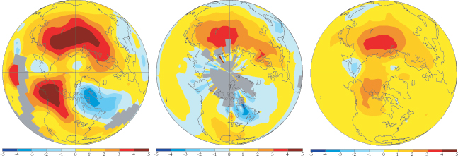
Observations show large increases in surface temperatures over the Northern Hemisphere (NH) continents during winter over the past few decades (Figure 1, left). Large areas have warmed at a rate more than an order of magnitude larger than the global annual average rate. These large changes appear to result largely from an increase in the westerly air flow around the NH, which brings warmer, wetter oceanic air over the continents and cooler interior air to the eastern coasts and the oceans. This westerly flow is associated with the leading variability pattern of NH cold season sea level pressure (SLP), called the "Arctic Oscillation" (AO) (Figure 1, middle). This oscillation is a hemispheric scale pattern which contains the North Atlantic Oscillation (NAO) in its Atlantic sector. Observations show an apparent upward trend in the amplitude of the AO pattern, or equivalently, a bias toward the positive phase of the pattern, in recent decades [Thompson and Wallace, 1998; Thompson et al., 2000]. The variability associated with this pattern extends from the surface up into the stratosphere, and in fact the variability pattern can be equivalently defined as being composed of variability at all levels from the surface through the lower stratosphere [Baldwin and Dunkerton, 1999]. The Goddard Institute for Space Studies (GISS) climate model is able to reproduce the observed trend in the AO in response to increasing greenhouse gases [Shindell et al., 1999a] only with the inclusion of a well-resolved stratosphere. Consistent with those results, observations indicate that changes in the stratospheric circulation typically precede the changes in the lower atmosphere [Kodera and Koide, 1997; Baldwin and Dunkerton, 1999]. As a result, the stratospheric climate model was better able to reproduce the large continental wintertime warming trends seen in the NH than a similar "tropospheric model" (Figure 1, right).
 |
||||
|
Figure 1. Surface temperature trends (&Mac251;C). (left) Observed surface temperature change
from 1965 to 1995, December to February average [Hansen et al., 1999]. (middle) The Arctic Oscillation (AO)
contribution to the total trend, obtained by regressing the temperature trend onto the AO spatial pattern
(as in the work by Thompson et al. [2000]). (Right) The AO component of the total trend in the GISS stratospheric
model, similarly obtained by regressing the model's temperature trend onto its AO spatial pattern. Grey areas
are those where no data is present. Note that the difference in grey areas between the left and middle maps results
from the use of slightly different temperature data sets, which do not match exactly in areas with few
observations (Arctic Ocean and low-latitude Atlantic and Pacific). |
||||
It is interesting to explore the various ways that stratospheric changes can influence tropospheric circulation.
For example, it has been shown that the circulation in the lower atmosphere can be affected by stratospheric changes
such as large volcanic eruptions [Rind et al., 1992; Graf et al., 1993; Kodera, 1994] or solar forcing [Haigh, 1999;
Shindell et al., 1999b]. But what is the mechanism by which stratospheric perturbations affect surface changes?
Greenhouse gas increases, volcanic aerosols, ozone depletion, or solar forcing can all induce meridional temperature
gradients in the stratosphere during wintertime. GCM experiments reveal a positive feedback whereby zonal wind
anomalies induced by these thermal gradients near the tropopause are amplified through planetary wave refraction.
Deflection of upward propagating tropospheric waves at lower and lower altitudes and the resulting changes in angular
momentum transport in effect carry the anomaly steadily down from the stratosphere, allowing stratospheric changes
to affect surface climate by altering tropospheric energy flow.
It is also useful to examine the extent to which each individual stratospheric forcing excites the natural patterns of variability. This is accomplished by projecting the induced changes onto empirical orthogonal functions (EOFs), fixed spatial patterns of variability ranked by the amount of variability accounted for by each pattern [e.g., Kutzbach, 1970], derived from a control run with no external forcings. In the observations, the recent trend in SLP has occurred primarily through enhancement of the AO (EOF 1) [Thompson et al., 2000]. In order to reproduce the observations, it is therefore necessary that a model yield a trend in the amplitude of the AO pattern similar to the observations, while at the same time keeping the amplitudes of changes in the other variability patterns small. The analysis of our model simulations shows that while greenhouse gas increases, volcanic aerosols, or Arctic ozone depletion can excite primarily this leading mode, only increasing greenhouse gases can excite an AO trend comparable to the observed value.
Several forcings may have contributed to surface climate change via the stratosphere. Increases have been observed in the abundance of atmospheric greenhouse gases, Arctic winter-spring ozone loss, and solar irradiance over decadal and longer time scales. While there is not thought to have been a long-term increase in volcanic eruptions, they can periodically cause very large perturbations to the stratosphere, providing an important test of the stratosphere's influence on surface climate. A systematic comparison of the mechanism by which perturbations to the stratosphere affect surface climate has been performed with the GISS GCM. Solar cycle variability is used here as a proxy for longer-term solar variations, which are not well constrained.
Empirical orthogonal functions (EOFs) were calculated from the NH cold season (November-April) sea-level pressure
(SLP) time series of the control run. The trend from the transient greenhouse gas runs was then projected upon those EOFs.
Other forcings were not run as transients, so differences between two states are used. For the solar cycle variability
simulations, the difference between the runs with solar maximum and solar minimum conditions was used. For the volcanic
forcing, the difference between the years when stratospheric aerosol loading was large (primarily the few years
immediately following eruptions) and years with background levels was used. Results for the ozone hole simulations
are differences between the simulation with polar heterogeneous chemistry included and a control run without the
chemistry parameterisation. For the transient simulations we define the time series corresponding to the leading EOF
as the "index" of the model's AO. The spatial pattern has been normalised so that the value of the AO index
is equal to the opposite of the SLP anomaly averaged poleward of 60°N, and is given in hPa. For the transient runs
the AO index trend is given over a 30-year period to match the observational record. The three-decade value we
present here was consistent for the entire five decades during which the AO increased steadily between the initial
spin-up and eventual saturation. For the tropospheric runs the averaging period has a minimal effect on the results,
as the trends were so small that no saturation was seen. For the solar, volcanic, and ozone hole simulations, whose
results are differences, we obtain a single value for the change in the AO index based upon the component of the
total SLP difference associated with the AO.
While the leading EOF is well separated from subsequent patterns, the higher EOFs are not adequately distinct from one another. In the stratospheric model forced with increasing greenhouse gases, EOF 1 accounts for 13.3% of the variance, but subsequent EOFs account for 5.9, 4.8, 4.1, and 3.5 percent, respectively, which are not statistically different within the calculated variance range of about 2% (calculations based on the entire 110 year run). An EOF analysis of the observations yields similar results, with 21.3, 11.7, 11.1, 8.2, and 7.0 percent variance explained by the first five EOFs (calculations based on 1947-1997 data). Again, only the leading pattern is well separated from the others. Since the higher modes are mathematical constructs which are forced to be orthogonal to the leading mode, not well separated, and lacking an obvious physical interpretation, we restrict our analysis to the leading EOF (the AO).
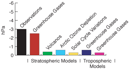
As discussed by Shindell et al. [1999a], the version of the GISS model containing a realistic representation of stratospheric processes produces an increasing AO trend in response to greenhouse gas increases of ~0.8 hPa/decade during the several decades between spin-up and saturation during which the AO index is increasing steadily. This value is comparable to the roughly 1 hPa/decade suggested by observations in recent decades. In contrast, model versions lacking a realistic stratosphere, "tropospheric models" with only one or two layers in the stratosphere, produce a leading EOF that also looks very much like the AO, but its index shows only a weak increasing trend (+0.1-0.3 hPa/decade) which is not statistically significant (Figure 2). It is interesting that when stratospheric water vapour is allowed to increase steadily, as a result of tropopause warming and methane oxidation [Shindell, 2001], this distinction between stratospheric and tropospheric models is slightly reduced. When water vapour and greenhouse gases both increase, the AO trend is reduced to ~0.6 hPa/decade, outside the range of the trend in the other three increasing greenhouse gas simulations (0.83, 0.78, and 0.79). This is due to the slight decrease in the meridional temperature gradient that results from mid-latitude cooling that ensues from water-vapour-induced ozone destruction in the lower stratosphere [Shindell, 2001]. Those simulations do not include the potential effect of increased water vapour on heterogeneous ozone destruction in the polar region, however, which would oppose the mid-latitude ozone-induced cooling and could potentially cause a significant increase in the meridional temperature gradient in the spring. Water vapour on its own, as a greenhouse gas, increases the bias toward the high phase of the AO.
 |
||||
| Figure 2. The magnitude of the trend or change in the AO index induced by each forcing. The magnitude of the AO is defined as the SLP anomaly averaged northward of 60 degrees. Values are calculated using a linear least squares regression through the observations or model output. Observations are updated from Trenberth and Paolino [1980]. | ||||
We find that the inclusion of an ozone hole in the model, another candidate for driving the observed increases [e.g., Graf et al.,
1998; Volodin and Galin, 1999], does cause an increase in the model's AO index, but of only ~0.6 hPa (1990s ozone
depletion relative to the 1970s and earlier, when there was no depletion, or approximately 0.3 hPa/decade over the
past two decades). Though this has likely contributed to the measured trend, it seems insufficient to account for a
great deal of the observed increase of several hPa over the past three decades. This is perhaps not surprising, since
the trend in the AO has been observed throughout the November-to-April cold season, but severe ozone depletion in
the Arctic does not take place in general until the spring, when sunlight falls on cold vortex air. This conclusion is in
agreement with the mild increase in the wintertime meridional temperature gradient at northern high latitudes
calculated using TOMS ozone trends [e.g., Ramaswamy et al., 1996]. While the TOMS observations were extrapolated
to high latitudes during the polar night, the use of in situ ozonesonde data [Randel and Wu, 1999a] does not change
this conclusion [Rosier and Shine, 2000]. This contrasts with the situation in the Antarctic, where ozone depletion
seems to account for nearly the entirety of the observed temperature trends [Randel and Wu, 1999b].
Volcanic forcing can be strong in the years immediately following an eruption, leading to an AO difference of 0.4 hPa between volcanic and non volcanic years, but since it is an intermittent forcing that decays rapidly, it also seems unlikely to have contributed greatly to the long-term observed trend. Solar cycle variability causes an increase in the AO index of 0.3 hPa between solar maximum and minimum. Since the longer-term trend in irradiance over the past 30 years has been of comparable size to solar cycle variability, it also seems unlikely that solar variability has been responsible for much of the observed trend. Furthermore, estimated solar irradiance increased as much in the first half of the twentieth century as in the second [Lean et al., 1997], but the AO index showed no increase during the former. However, the long-term response would include a response of the ocean to solar forcing, while the shorter-term solar cycle does not, so that the response may in fact be somewhat different over longer time scales.
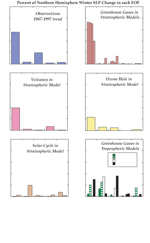
The stratosphere model is distinct from the tropospheric models not only for exhibiting a trend of magnitude comparable to the observed value, but because the spatial distribution of its SLP trend closely resembles the AO spatial pattern, as observed [Thompson and Wallace, 1998]. The resemblance of the SLP trend to the AO spatial pattern can be quantified by decomposing the trend into the EOFs of SLP and measuring the contribution of each EOF to the trend variance (Figure 3), following Fyfe et al. [1999]. The trend in observations of cold season SLP between 1967 and 1997 [Trenberth and Paolino, 1980, updated to 1997] is dominated by a change in the AO (the leading EOF), which contributes 56% of the trend. The GISS stratospheric model with increasing greenhouse gases puts 64% of the trend in the AO (the average value of the ensemble of four simulations). The stratospheric model with either an ozone hole or volcanic forcing also projects primarily onto the first EOF; however, solar cycle variability does not. The stratospheric model with increasing water vapour projects less strongly onto the AO than do the other increasing greenhouse gas runs, but its trend is still dominated by the AO (and actually looks most like the observed trend projections).
 |
||||
| Figure 3. Percentage of the total Northern Hemisphere November-April sea level pressure change in each empirical orthogonal function (EOF). Trends from each indicated model simulation were projected upon EOFs taken from the control run. Observations are updated from Trenberth and Paolino [1980], as in Figure 2. | ||||
In contrast, GISS model versions lacking a detailed stratosphere ("tropospheric models") forced with increasing greenhouse gases produce trends that project only 5-20% onto the AO (Figure 3). The GISS tropospheric model including sulphate aerosols puts just 6% of its trend into the leading EOF, with most of its trend spread out over a large number of patterns. Transient greenhouse gas experiments by other modelling groups seem to be consistent with this distinction (Figure 3). The Canadian Climate Center CCCma model [Fyfe et al., 1999], which shows a positive AO trend in response to increasing greenhouse gases despite the absence of detailed stratospheric dynamics, similarly fails to reproduce the observed dominance of the AO pattern, putting less than 30% of its total trend into its leading EOF. A Geophysical Fluid Dynamics Laboratory (GFDL) climate model version lacking a detailed stratosphere also finds that the majority of its SLP trend in response to increasing greenhouse gases is not in the AO (P. Kushner, personal communication, 1999). Several other groups have presented the simulated AO response to increasing greenhouse gases. The ECHAM3 model from the Max Planck Institute for Meteorology, without a full representation of the stratosphere, shows a systematic increase in the AO index in response to increasing greenhouse gases [Graf et al., 1995, 1998; Perlwitz et al., 2000], but its amplitude is stated to be weaker than observed. Paeth et al. [1999] present results of simulations with both the ECHAM3 and ECHAM4 models (showing NAO trends, but these are likely very similar to AO trends). Zorita and Gonzalez-Rouco [2000] present the AO trends from the same simulations, adding in results from the Hadley Center model 2 as well. Along with Fyfe et al. [1999], all of these groups use normalised units to present their trends, making it impossible to compare the magnitude of the increase in those simulations to the observed value. We suggest that documentation of a model's AO trend should include, at minimum (1) the trend's magnitude in hPa and its statistical significance, with a description of the area weighting used, and (2) the decomposition of the trend into its component EOFs. This information would facilitate a comparison across models to document more clearly the role of stratospheric dynamics. As yet, only models that realistically simulate the stratosphere have quantitatively demonstrated an AO trend of roughly the right magnitude and with the same predominance within the SLP trend as the observations.
The upper troposphere in the tropics warms significantly in response to increases in greenhouse gases. This leads to a sharp contrast with latitude in the temperature response in the tropopause region. While the upper troposphere is closely connected to the surface by moist convective processes at low latitudes, and therefore warms, the same altitudes lie within the stratosphere at higher latitudes, as the height of the tropopause decreases abruptly poleward of the mid-latitude jet. Increasing greenhouse gases cool the stratosphere, and therefore enhance the meridional temperature gradient across the jet core. This gradient increase, which is largely zonally symmetric, is associated with strengthened westerlies within the jet. The strengthened mid-latitude jet alters the propagation of planetary waves, which can potentially feed back on the jet through eddy forcing.
Volcanic forcing is similar, as aerosol heating in the sunlit portion of the winter atmosphere warms that region relative to the part of the atmosphere in polar darkness, enhancing the latitudinal temperature gradient. Arctic ozone depletion does the same thing too, as less ozone at high latitudes leads to a cooling there due to the reduction in short-wave absorption by ozone. This happens much later than the others, however, as sunlight returns to high latitudes and ozone depletion takes place only in the spring around March and April, so that this has a relatively small impact over the entire November-to-April cold-season, and no real effect during December-to-February.
Amplification by planetary waves is largest in NH winter, when planetary wave activity is greatest. While we used
the November-April cold season for SLP, to facilitate comparison with other analyses of the AO, we return now to the
conventional December-February winter period for easier comparison with model output and with observations of more
standard meteorological parameters. Planetary wave refraction is governed by wind shear, among other factors, so that
enhanced wave refraction occurs as the waves approach the area of increased wind speed. In this case, since planetary
waves are propagating up from the surface, they are refracted by the increased vertical shear below the enhanced zonal
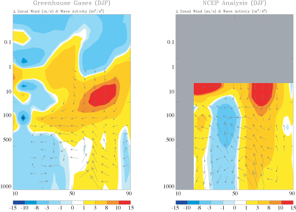
wind. Equatorward refraction of planetary waves at the lower edge of the wind anomaly (Figure 4) leads to
wave divergence and hence an acceleration of the zonal wind in that region. Over time, the wind anomaly itself thus
propagates downward [Haynes et al., 1991] from the lower stratosphere to the surface.
 |
|||
| Figure 4. Trends in zonal mean zonal wind (m/s) and planetary wave activity (m2/s2) (left) in the greenhouse gas simulations and (right) in analysed observations. Model trends are shown for the five decades during which the AO increased steadily between the initial spin-up and eventual saturation (1980-2030). Observed trends are differences between the high-AO years 1981, 1983, and 1984 and the low-AO years 1979, 1982, and 1992 using NCEP analyses of observational data. Values are the sum of the total trend components in the first two EOFs of these trends, as given by Ohhashi and Yamazaki [1999, Figures 7 and 8] (Hartmann et al. [2000] show similar results). Since the first two EOFs contain nearly all the variability, these should be comparable to the model's total trend values. Vertical fluxes have been scaled by the inverse of pressure for convenience in all plots. The maximum vector length corresponds to 7 m2/s2. The total AO index change in the model over this five-decade period was about 4 hPa, somewhat larger than the 1979 to 1992 variability of about 2.5 hPa. | |||
The precise location of the enhanced westerlies shown in Figure 4 therefore depends upon the interaction between planetary
waves, wind shears, eddy fluxes and angular momentum fluxes, and is not a simple function of the location of the strongest
temperature contrast. This is likely the cause of the difference in location between the strongest enhancement of the
temperature gradient, which is at the latitude of the jet stream, and the location of the strongest zonal wind enhancement,
which is at the latitude of the polar night jet. Further work will be required to fully elucidate the link between the
meridional structures of the temperature and wind responses to external forcing.
The overall equatorward refraction of planetary waves and reduced upward propagation at high latitudes shown
in Figure 4 affect the location of wave dissipation. The net result is a reduced ability of individual waves to
abruptly enhance the residual circulation and create sudden warmings. In fact, there is a strong anticorrelation
between the frequency of sudden stratospheric warmings and the AO index strength [Hartmann et al., 2000].
The behaviour of the troposphere is in accord with theory stating that angular momentum is in general transported in the opposite meridional direction to planetary wave energy [Andrews et al., 1987]. In this case, angular momentum is then preferentially transported poleward, enhancing westerlies, as waves are refracted towards the equator in the upper troposphere. Geostrophic and hydrostatic balance in the atmosphere is maintained by generation of a vertical circulation cell consistent with the northerly angular momentum transfer. Increased westerlies are transformed into northerly flow by surface friction, leading to a cell with rising air in the polar region, and descending air at middle latitudes from about 40° to 55°N throughout the troposphere and the lower stratosphere. The effects are clearly visible in the SLP field as a decrease in the Arctic concurrent with increased mid-latitude pressure. Adiabatic expansion of rising air at high latitudes must be balanced by radiative heating, which occurs as a result of further cooling of the air below its radiative equilibrium temperature. Conversely, sinking air at mid-latitudes warms. The increased latitudinal temperature gradient that results is consistent with the increased westerly zonal wind around 55°N seen in the model and in observations [Baldwin and Dunkerton, 1999; Thompson et al., 2000]. The surface wind anomaly is therefore created by the effect of the increased lower stratospheric zonal wind on planetary waves via linked changes in planetary wave and angular momentum fluxes. It is this increase in surface wind that leads to greater advection of warm oceanic air over the downstream continents. The role of the stratosphere in influencing the behaviour of surface meteorology in the model is in agreement with the observed co-variability between the lower stratosphere and the surface [e.g., Perlwitz and Graf, 1995; Graf et al., 1995; Thompson and Wallace, 1998]. It is also consistent with the large role played by planetary waves in creating the AO pattern itself during midwinter in the NH, as evidenced by the fact that the AO structure amplifies with height up into the stratosphere only during this season, when the zonal flow is conducive to strong wave-mean flow interaction [Baldwin and Dunkerton, 1999; Thompson and Wallace, 2000]. This would also explain why there has only been an upward trend in the AO during NH winter.
The model simulations have shown that a surface climate response is induced by increasing greenhouse gases,
ozone depletion, volcanic eruptions, and solar variability. Except for solar variability, the others all affect surface
climate at NH middle and high latitudes during winter primarily by favouring the positive phase of the AO, the dominant
natural variability pattern, while concurrently strengthening the polar vortex aloft. Nonetheless, only increasing
greenhouse gases seem capable of causing an AO trend in our model as large as the observed trend.
The AO sensitivity of models developed by several groups, including GISS, which lack realistic representations
of the stratosphere, is much weaker than the GISS stratospheric model. It seems that models with an overly
simplistic stratosphere fail to adequately capture the positive feedback of planetary wave flux changes on
circulation anomalies seen in the stratospheric model. Furthermore, the simulated trends in those models
are not primarily composed of the AO pattern, as are the observations, while the stratospheric model
does reproduce this behaviour.
The surface climate response of the GISS stratospheric model to the injection of volcanic aerosols into
the stratosphere corresponds well with observations. This provides important evidence that the modelled
linkage between forcings and the AO does indeed occur in the atmosphere. While longer-term AO changes
will need to continue for many more years to be fully accepted as a distinct trend, the AO enhancement
after eruptions is already quite clear in the observational record. Since the AO responses to greenhouse
gas increases, ozone depletion, and volcanic aerosols all take place via the same mechanism, the clearly
observed response to large volcanic eruptions suggests that the same linkage is likely at work in the case
of the slower, longer-term greenhouse gas and ozone depletion forcings as well.
An obvious question is how would the response vary from model to model, using models with a realistic stratosphere? There are likely to be considerable intermodel variations, as one of the dominant factors controlling the sensitivity of the AO to forcings is the surface temperature response to forcings, which differs considerably between models [IPCC, 1995]. The magnitude of the tropical surface warming seems to play a major role in changes in the latitudinal temperature gradient via its control over warming in the tropical upper troposphere. The degree of this warming is probably the largest uncertainty in the overall magnitude of the change in the latitudinal temperature gradient, as the stratospheric cooling is purely radiative, and similar in most models [e.g., WMO, 1999]. Thus the tropical surface warming directly governs a significant part of the AO in response to climate forcings. This implies that the surface response is crucial to the stratospheric response, an interesting variation on the stratosphere-climate linkages that are the focus of SPARC. These interactions clearly go in both directions.
Andrews, D. G., J. R. Holton, and C. B. Leovy, Middle Atmosphere Dynamics, 489 pp., Academic, San Diego,
Calif., 1987.
Baldwin, M. P., and T. J. Dunkerton, Propagation of the Arctic Oscillation from the stratosphere to the troposphere, J. Geophys. Res., 104,30,937-30,946, 1999.
Fyfe, J. C., G. J. Boer, and G. M. Flato, The Arctic and Antarctic Oscillations and their projected changes under global warming, Geophys. Res. Lett., 26, 1601-1604, 1999.
Graf, H.-F., I. Kirchner, A. Robock, and I. Schult, Pinatubo eruption winter climate effects: Model versus observations , Clim. Dyn., 9, 81-93, 1993.
Graf, H.-F., J. Perlwitz, I. Kirchner, and I. Schult, Recent northern winter climate trends, ozone changes and increased greenhouse gas forcing, Beitr. Phys. Atmos., 68, 233-248, 1995.
Graf, H.-F., I. Kirchner, and J. Perlwitz, Changing lower stratospheric circulation: The role of ozone and greenhouse gases, J. Geophys. Res., 103, 11,251-11,261, 1998.
Haigh, J. D., A GCM study of climate change in response to the 11-year solar cycle, Q. J. R. Meteorol. Soc., 125, 871-892, 1999.
Hansen, J., R. Ruedy, J. Glascoe, and M. Sato, GISS analysis of surface temperature change, J. Geophys. Res., 104, 30,997-31,022, 1999.
Hartmann, D. L., J. M. Wallace, V. Limpasuvan, D. W. J. Thompson, and J. R. Holton, Can ozone depletion and global warming interact to produce rapid climate change, Proc. Natl. Acad. Sci., 97, 1412-1417, 2000.
Haynes, P. H., C. J. Marks, M. E. McIntyre, T. G. Shepherd, and K. P. Shine, On the "downward control" of extratropical diabatic circulation by eddy-induced mean zonal forces, J. Atmos. Sci., 48, 651-678, 1991.
International Panel on Climate Change (IPCC), Climate Change, 1995, edited by J. T. Houghton et al., 572 pp., Cambridge Univ. Press, New York, 1996.
Kodera, K., Influence of volcanic eruptions on the troposphere through stratospheric dynamical processes in the Northern Hemisphere winter, J. Geophys. Res., 99, 1273-1282, 1994
Kodera, K., and H. Koide, Spatial and seasonal characteristics of recent decadal trends in the Northern Hemisphere troposphere and stratosphere, J. Geophys. Res., 102, 19,433-19,447, 1997.
Kutzbach, J. E., Large-scale features of monthly mean Northern Hemisphere anomaly maps of sea-level pressure, Mon. Weather Rev., 98, 708-716, 1970.
Labitzke, K., and H. van Loon, The signal of the 11-year sunspot cycle in the upper troposphere- lower stratosphere, Space Sci. Rev., 80, 393-410, 1997.
Lean, J. L., G.J. Rottman, H.L. Kyle, T.N. Woods, J.R. Hickey, and L.C. Puga, Detection and parameterization of variations in solar mid- and near-ultraviolet radiation (200-400 nm), J. Geophys. Res., 102, 29,939-29,956, 1997.
Ohhashi, Y., and K. Yamazaki, Variability of the Eurasian pattern and its interpretation by wave activity flux, J. Meteorol. Soc. Jpn., 77, 495-511, 1999.
Paeth, H., A. Hense, R. Glowienka-Hense, R. Voss, and U. Cubash, The North Atlantic Oscillation as an indicator for greenhouse-gas induced regional climate change, Clim. Dyn., 15, 953-960, 1999.
Perlwitz, J., and H.-F. Graf, The statistical connection between tropospheric and stratospheric circulation of the Northern Hemisphere in winter, J. Clim., 8, 2281-2295, 1995.
Perlwitz, J., H.-F. Graf, and R. Voss, The leading variability mode of the coupled troposphere-stratosphere winter circulation in different climate regimes, J. Geophys. Res., 105, 6915-6926, 2000.
Ramaswamy, V., M. D. Schwarzkopf, and W. J. Randel, Fingerprint of ozone depletion in the spatial and temporal pattern of recent lower-stratospheric cooling, Nature, 382, 616-618, 1996.
Randel, W. J., and F. Wu, A stratospheric ozone trends data set for global modelling studies, Geophys. Res. Lett., 26, 3089-3092, 1999a.
Randel, W. J., and F. Wu, Cooling of the arctic and antarctic polar stratospheres due to ozone depletion, J. Clim., 12, 1467-1479, 1999b.
Rind, D., N. K. Balachandran, and R. Suozzo, Climate change and the middle atmosphere, II, The impact of volcanic aerosols, J. Clim., 5, 189-208, 1992.
Rosier, S. M., and K. P. Shine, The effect of two decades of ozone change on stratospheric temperature as indicated by a general circulation model, Geophys. Res. Lett., 27, 2617-2620, 2000.
Shindell, D. T., R. L. Miller, G. A. Schmidt, and L. Pandolfo, Simulation of recent northern winter climate trends by greenhouse gas forcing, Nature, 399, 452-455, 1999a.
Shindell, D. T., D. Rind, N. Balachandran, J. Lean, and P. Lonergan, Solar cycle variability, ozone, and climate, Science, 284, 305-308, 1999b.
Shindell, D. T., Global warming due to increased stratospheric water vapour, Geophys. Res. Lett., 28, 1551-1554, 2001.
Thompson, D. W. J., and J. M. Wallace, The Arctic Oscillation signature in the wintertime geopotential height and temperature fields, Geophys. Res. Lett., 25, 1297-1300, 1998.
Thompson, D. W. J., and J. M. Wallace, Annular modes in the extratropical circulation, I, Month-to-month variability, J. Clim., 13, 1000-1016, 2000.
Thompson, D. W. J., J. M. Wallace, and G. C. Hegerl, Annular modes in the extratropical circulation, II, Trends, J. Clim., 13, 1018-1036, 2000.
Trenberth, K. E., and D. A. Paolino, The Northern Hemisphere sea level pressure data set: Trends, errors, and discontinuities, Mon. Weather Rev.,108, 855-872, 1980.
Volodin, E. M., and V. Y. Galin, Interpretation of winter warming on Northern Hemisphere continents in 1977-94, J. Clim., 12, 2947-2955, 1999.
World Meteorological Organization, Scientific Assessment of Ozone Depletion: 1998, Rep. 44, Geneva, 1999.
Zorita, E., and F. Gonzalez-Rouco, Disagreement between predictions of the future behavior of the Arctic Oscillation
as simulated in two different climate models: Implications for global warming, Geophys. Res. Lett., 27, 1755-1758, 2000.
![]()