 |
Stratospheric Processes And their Role in Climate
|
||||||||
| Home | Initiatives | Organisation | Publications | Meetings | Acronyms and Abbreviations | Useful Links |
![]()
|
Stratospheric Processes And their Role in Climate
|
||||||||
| Home | Initiatives | Organisation | Publications | Meetings | Acronyms and Abbreviations | Useful Links |
![]()
The strength of the wintertime vortex is reflected in polar temperature, which undergoes large variations between years. So does total ozone at extratropical latitudes. Both are regulated by the residual mean circulation of the middle atmosphere. Air descending at high latitudes of the winter hemisphere experiences adiabatic warming that offsets radiative cooling, maintaining wintertime temperatures well above radiative equilibrium. Residual mean motion also transfers ozone poleward and downward, its column abundance increasing steadily during winter until reaching its spring maximum.
Interannual changes are an important focus of stratospheric research. Understanding them is necessary to properly identify anthropogenic changes. Interannual changes of dynamical structure over the 1980s and 1990s have been studied in global analyses from ECMWF. Dynamical changes in the lower stratosphere (LS) are investigated in relation to contemporaneous changes of total ozone from TOMS, likewise concentrated in the LS. These changes of dynamical and chemical structure are then related to interannual changes of temperature and ozone in the upper stratosphere observed by the French lidar at Observatoire de Haute-Provence (OHP).
Figure 1 shows the mean annual cycle of column-averaged temperature at 100-10hPa over the Arctic T (solid), which has been constructed by averaging ECMWF analyses over the years 1979-1998. Following summer solstice, polar temperature decreases steadily until reaching a minimum shortly after winter solstice. Interannual variance of polar temperature (shaded) has similar seasonality, increasing sharply during the disturbed months of winter. Planetary waves propagating upward from the troposphere at this time of year drive downwelling over the Arctic, which introduces adiabatic warming.
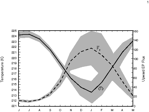
Figure 1. Mean annual cycle of column-averaged temperature above 100hPa (solid) and upward EP flux at 100hPa (dashed), normalised, each averaged over 50°N-90°N, along with the std. deviation of their interannual variability (shaded).
Superposed in Figure 1 is the mean annual cycle of upward EP flux
at 100hPa ![]() (dashed), averaged over the northern extratropics. It represents
westward momentum that is transmitted upward from the troposphere
by planetary waves and is largely absorbed in the middle atmosphere.
As such,
(dashed), averaged over the northern extratropics. It represents
westward momentum that is transmitted upward from the troposphere
by planetary waves and is largely absorbed in the middle atmosphere.
As such, ![]() measures overall wave driving of the residual mean circulation
and thus downwelling over the Arctic, where adiabatic warming
offsets radiative cooling.
measures overall wave driving of the residual mean circulation
and thus downwelling over the Arctic, where adiabatic warming
offsets radiative cooling. ![]() has seasonality just opposite to
has seasonality just opposite to ![]() , maximising shortly after winter solstice, when perpetual darkness
over the Arctic leads to strong LW cooling. The interannual variance
of
, maximising shortly after winter solstice, when perpetual darkness
over the Arctic leads to strong LW cooling. The interannual variance
of ![]() (shaded) has similar seasonality. Largest changes of upward EP
flux from the troposphere are observed during the dynamically-disturbed
season.
(shaded) has similar seasonality. Largest changes of upward EP
flux from the troposphere are observed during the dynamically-disturbed
season.
The annual cycle of ![]() implies strong adiabatic warming during winter that offsets strong
LW~cooling, controlling the minimum polar temperature that is
achieved each year around solstice. By driving residual mean motion
that transfers ozone-rich air poleward and downward,
implies strong adiabatic warming during winter that offsets strong
LW~cooling, controlling the minimum polar temperature that is
achieved each year around solstice. By driving residual mean motion
that transfers ozone-rich air poleward and downward, ![]() also controls the spring maximum of total ozone. About their mean
annual cycles, temperature, ozone, and upward EP flux from the
troposphere each experience sizeable changes from one year to
the next. Over the two decades under consideration, those changes
define a cloud of some 20 realisations of the annual cycle, as
characterised by the rms variation in Figure 1 (shaded). Each
realisation of the annual cycle determines the interannual anomaly, defined as the deviation from the 20-year mean annual variation.
In the analysis below, we explore how the anomaly during an individual
year in one of these properties is related to the anomaly during
the same year in the other properties.
also controls the spring maximum of total ozone. About their mean
annual cycles, temperature, ozone, and upward EP flux from the
troposphere each experience sizeable changes from one year to
the next. Over the two decades under consideration, those changes
define a cloud of some 20 realisations of the annual cycle, as
characterised by the rms variation in Figure 1 (shaded). Each
realisation of the annual cycle determines the interannual anomaly, defined as the deviation from the 20-year mean annual variation.
In the analysis below, we explore how the anomaly during an individual
year in one of these properties is related to the anomaly during
the same year in the other properties.
Interannual changes of wintertime temperature are large over the polar cap. Their vertical structure is deep. Figure 2a shows the anomalous wintertime temperature during January 1980. It's large over the Arctic, where anomalous temperature is uniformly negative (January temperatures colder than average). Anomalous temperature increases upward to the roof of the ECMWF analyses, amplifying to more than 7 K by 10hPa. At sub-polar latitudes, it has reversed sign, but it's much smaller. Over the equator, values are dominated by the temperature signature of the QBO, which is out of phase between 70 and 30hPa.
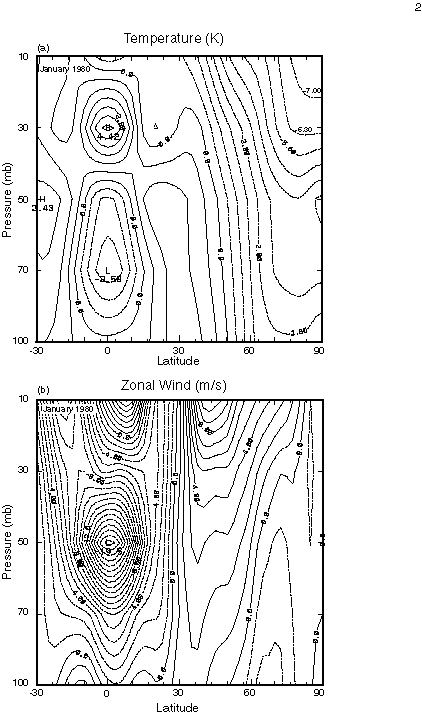
Figure 2. (a) Anomalous zonal-mean temperature, as a function of latitude and pressure, for January 1980. (b) As in (a), but for zonal-mean wind.
Zonal-mean wind is shown in Figure 2b, also for January 1980. Anomalous wind is positive at high latitudes, westerlies increasing upward along the axis of the polar-night jet to the highest level represented in the analyses. In the tropics, QBO easterlies prevail over the entire LS. This distribution of equatorial wind displaces the critical line of planetary waves into the winter hemisphere, favouring wave absorption farther northward and a polar-night vortex that is anomalously warm and weak (Holton and Tan, 1980; Labitzke, 1982). Yet, during this particular year, the January vortex is actually anomalously cold and strong.
During the winter in Figure 2, upward EP flux from the troposphere
is anomalously weak (not shown). This implies a residual circulation
during 1980 that is likewise anomalously weak. Through reduced
downwelling and adiabatic warming, anomalously-weak ![]() also implies a polar-night vortex that is anomalously cold and
strong -- as is observed.
also implies a polar-night vortex that is anomalously cold and
strong -- as is observed.
The correspondence during 1980 between anomalous temperature and
wave driving by the troposphere, in fact, reflects a more general
relationship. Figure 3 compares the anomalous column-averaged temperature over the Arctic
during January (solid), as a function of year, against the corresponding
record of anomalous ![]() (dashed), integrated over the northern extratropics and during
the preceding months of winter. The latter represents the cumulative
wave driving of residual motion leading up to the temperature
minimum in January. The relationship is clear and it's strong:
Interannual changes of temperature over the Arctic closely track
interannual changes of westward momentum transmitted to the middle
atmosphere by planetary waves. With a correlation of 0.89, changes
of
(dashed), integrated over the northern extratropics and during
the preceding months of winter. The latter represents the cumulative
wave driving of residual motion leading up to the temperature
minimum in January. The relationship is clear and it's strong:
Interannual changes of temperature over the Arctic closely track
interannual changes of westward momentum transmitted to the middle
atmosphere by planetary waves. With a correlation of 0.89, changes
of ![]() account for almost all of the interannual variance of minimum
polar temperature.
account for almost all of the interannual variance of minimum
polar temperature.
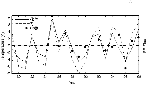
Figure 3. Anomalous column-averaged (100-10hPa) temperature during January (60°N-90°N), as a function of year, compared against the anomalous upward EP flux from the troposphere (50°N-90°N) integrated over the preceding months Jan.-Oct. (normalised). Superposed is the column-averaged temperature above 30km (circles) during January, observed at OHP.
The structure of interannual changes has been composited from
its spatial coherence, with 100hPa temperature over the North
Pole serving as a reference time series. Figure 4 shows the anomalous January temperature corresponding to a 1-std
deviation increase of ![]() . Like anomalous structure during 1980, it's deep -- significant
at the 95\% level (shaded) over most of the winter hemisphere.
Anomalous temperature is strong over the Arctic, where positive
values reflect enhanced downwelling and adiabatic warming. It
increases upward, approaching 7 K near 30hPa. That's close to
the overall std deviation of polar temperature in the LS, as changes
operating coherently in the vertical account for nearly all of
its interannual variance. South of 50°N, anomalous temperature
is negative, reflecting enhanced upwelling and adiabatic cooling.
However, although just as significant as changes at high latitudes,
temperature changes in the tropics are an order of magnitude weaker.
. Like anomalous structure during 1980, it's deep -- significant
at the 95\% level (shaded) over most of the winter hemisphere.
Anomalous temperature is strong over the Arctic, where positive
values reflect enhanced downwelling and adiabatic warming. It
increases upward, approaching 7 K near 30hPa. That's close to
the overall std deviation of polar temperature in the LS, as changes
operating coherently in the vertical account for nearly all of
its interannual variance. South of 50°N, anomalous temperature
is negative, reflecting enhanced upwelling and adiabatic cooling.
However, although just as significant as changes at high latitudes,
temperature changes in the tropics are an order of magnitude weaker.
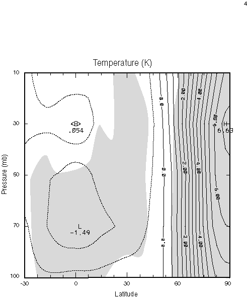
Figure 4. Anomalous January temperature, as a function of latitude and pressure, operating coherently with 100hPa temperature over the North Pole. 95%-significance level shaded.
The smallness of temperature changes in the tropics has been argued as evidence for no change of the residual circulation, leaving much larger changes at high latitudes to be associated with changes of ozone (WMO, 1999). However, temperature changes in the tropics operate coherently with changes at high latitudes. Their disparate magnitude reflects two basic features of the residual circulation: (1) Temperature tendencies at high latitudes are emphasised by spherical geometry, which leads to strong downwelling and adiabatic warming over the pole, but much weaker upwelling and adiabatic cooling at low latitudes. (2) In polar darkness, radiative damping is slow enough for descending air to warm adiabatically with little diabatic loss, in contrast to faster radiative damping that operates on ascending air in illuminated regions.
Interannual changes in the LS are accompanied by changes in the upper stratosphere and mesosphere. Those changes are observed by the lidar at OHP, which retrieves temperature above 30km via Rayleigh scattering (Hauchecorne and Chanin, 1980; Keckhut et al., 1995). Superposed in Figure~3 is the anomalous column-averaged temperature above 30km observed at OHP (solid circles). These are local measurements, in contrast to the horizontally-averaged behaviour from ECMWF. Some years are missing due to limited sampling. Note also that OHP, situated at 44°N, lies well south of the polar cap, where temperatures from ECMWF (solid) have been averaged. Despite these limitations, the OHP record is strongly correlated to temperature changes in the LS. In years when the Arctic LS is anomalously warm, so too is the upper stratosphere above OHP. Just the reverse is observed in years when the Arctic LS is anomalously cold.
Figure 5 shows the vertical structure of anomalous temperature at OHP (solid), which has been composited from its vertical coherence. Anomalous temperature is positive from 30 to 60km (January temperatures warmer than average), where it is 95% significant and changes coherently with temperature in the Arctic LS. Above 60km, temperature also changes coherently with temperature in the LS, but out of phase.
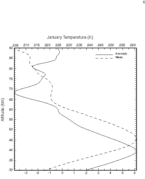
Figure 5. Anomalous January temperature at OHP (solid), as a function of altitude, composited against temperature changes at 40km. Also shown is the 20-year mean January temperature at OHP (dashed).
The structure of temperature changes above 30km resembles mean thermal structure (dashed), which is superposed in Figure 5. Both increase upward to about 45km and then decrease into the mesosphere. The profile of anomalous temperature is displaced downward relative to mean temperature by ~ 5km, reflecting downwelling that tends to lower isotherms. Anomalous temperature reverses sign above 60km. This happens to be the level where the meridional gradient of temperature reverses: coldest temperatures found over the winter pole in the stratosphere, but over the summer pole in the mesosphere. The similarity of temperature profiles in Figure 5 implies that interannual changes at OHP result principally from changes of meridional transport, which lead to a meridional swing of isotherms: OHP is positioned equatorward of strong downwelling over the Arctic and, hence, where residual motion is dominated by poleward transport. During winters when the meridional circulation is strong, warmer isotherms south of OHP and in the stratosphere expand poleward, as the vortex recedes. This is observed at OHP as a shift of stratospheric temperatures to warmer values. In the mesosphere, however, colder isotherms south of OHP expand poleward, shifting temperatures at OHP to colder values. During winters when the residual circulation is weak, just the reverse occurs.
Figure 6 plots the anomalous 100hPa height during January, which has been composited from its spatial coherence with 50hPa height over the North Pole. Anomalous height is strong and positive over the Arctic, where it weakens the polar low and upper-tropospheric westerlies during January. Positive values reflect enhanced downwelling and adiabatic warming, driven by anomalous wave absorption during winters when upward EP flux from the troposphere is enhanced. Surrounding the positive anomaly over the Arctic is negative anomalous height at mid-latitudes. It's concentrated over the north Atlantic, between Europe and North America, and over the north Pacific, between Asia and North America. Like the stronger anomaly over the Arctic, these mid-latitude changes are 95% significant, so they operate coherently with changes of opposite sign over the polar cap.
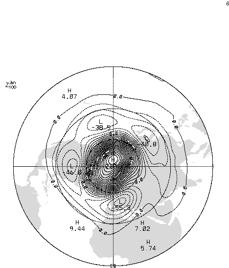
Figure 6. Anomalous January 100hPa height, composited against 50hPa height over the North Pole.
The anomalous structure in Figures 4 and 6 shares certain features
with the so-called Arctic Oscillation (AO) (Wallace and Thompson,
1998; 2000); see the recent review by Baldwin (2000). Derived
from the leading EOF of sea-level presure (SLP), the AO involves temperature changes that maximise over
the Arctic in the LS. They decrease sharply at subpolar latitudes,
where anomalous temperature has opposite sign and remains comparatively
small. Despite these similarities, temperature changes operating
coherently with![]() are deeper than those operating coherently with SLP. They remain
strongly coherent to the highest level represented in ECMWF analyses.
More importantly, changes in Figure 4 are 2-3 times stronger than
changes operating coherently with SLP. These differences imply
contributions to anomalous wintertime temperature other than those
represented in the leading EOF of SLP. They also reflect the very
high spatial coherence of stratospheric temperature and its coherence
to
are deeper than those operating coherently with SLP. They remain
strongly coherent to the highest level represented in ECMWF analyses.
More importantly, changes in Figure 4 are 2-3 times stronger than
changes operating coherently with SLP. These differences imply
contributions to anomalous wintertime temperature other than those
represented in the leading EOF of SLP. They also reflect the very
high spatial coherence of stratospheric temperature and its coherence
to ![]() (Figure 2),
(Figure 2),
The annual cycle of total ozone is lagged with respect to the annual cycle of polar temperature by 3~months, reflecting the additional time for ozone to be exported poleward. Analogous to polar temperature, its interannual variance is large during winter months leading up to its maximum, which is reached shortly after spring equinox.
Figure 7 compares the record of anomalous March ozone from TOMS (solid),
averaged over the northern extratropics, against the corresponding
record of ![]() (dashed), integrated over the preceding months of winter. Like
polar temperature, interannual changes of spring ozone track changes
of upward EP flux from the troposphere. In years when
(dashed), integrated over the preceding months of winter. Like
polar temperature, interannual changes of spring ozone track changes
of upward EP flux from the troposphere. In years when ![]() is anomalously strong, March ozone is anomalously large. Just
the reverse is observed in years when
is anomalously strong, March ozone is anomalously large. Just
the reverse is observed in years when ![]() is anomalously weak. It's noteworthy that this relationship holds
even in years of unusually low ozone, like 1997.
is anomalously weak. It's noteworthy that this relationship holds
even in years of unusually low ozone, like 1997.
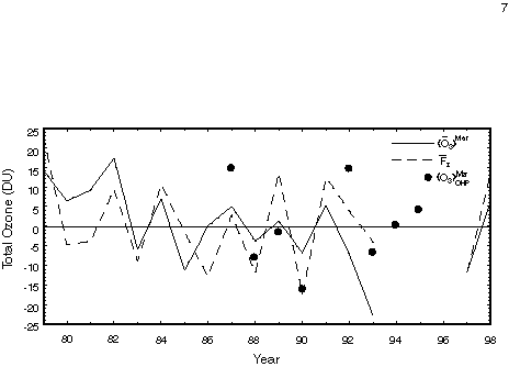
Figure 7. Anomalous March total ozone (10°N-90°N), as a function of year, compared against the anomalous upward EP flux from the troposphere (55°N-90°N) during Dec.-Feb. (normalised). Also shown is the anomalous column abundance above 30km during March observed at OHP (normalised).
While being strongly correlated to spring ozone, interannual changes
of ![]() do not account for all of its variance -- in contrast to interannual
changes of minimum polar temperature observed during early winter
(Figure 2). Other mechanisms also contribute to interannual changes
of spring ozone. A similar conclusion applies to spring temperature,
which tracks the record of
do not account for all of its variance -- in contrast to interannual
changes of minimum polar temperature observed during early winter
(Figure 2). Other mechanisms also contribute to interannual changes
of spring ozone. A similar conclusion applies to spring temperature,
which tracks the record of ![]() is similar fashion.
is similar fashion.
Interannual changes of ![]() reflect changes in overall wave driving of the residual circulation.
The residual circulation is influenced as well by the QBO, which
controls where wave activity is absorbed (e.g., Tung and Yang,
1994). By doing so, the QBO also affects mean downwelling over
the winter hemisphere and, thus, springtime temperature and ozone.
Another source of interannual variance comes from volcanic perturbations,
during the years immediately following El Chichon and Pinatubo.
They alter diabatic heating and ozone photochemistry (WMO, 1995),
but occupy only a small fraction of the overall record.
reflect changes in overall wave driving of the residual circulation.
The residual circulation is influenced as well by the QBO, which
controls where wave activity is absorbed (e.g., Tung and Yang,
1994). By doing so, the QBO also affects mean downwelling over
the winter hemisphere and, thus, springtime temperature and ozone.
Another source of interannual variance comes from volcanic perturbations,
during the years immediately following El Chichon and Pinatubo.
They alter diabatic heating and ozone photochemistry (WMO, 1995),
but occupy only a small fraction of the overall record.
Like interannual changes of temperature, interannual changes of
ozone are strong at high latitudes. Figure 8 shows the structure of anomalous March ozone, as a function of
latitude, which has been composited from its spatial coherence.
Anomalous ozone is positive in the extratropics, where it reflects
enhanced downwelling of ozone-rich air during winters when ![]() is anomalously strong. It approaches 25 DU at high latitudes,
where anomalous temperature is also positive and strong. In the
tropics, anomalous ozone has opposite sign, reflecting enhanced
upwelling of ozone-lean air during the same winters. Compensating
changes at high and low latitudes also appear in zonal-mean ozone
structure observed by MLS (Fusco and Salby, 1999). Like temperature
changes, however, ozone changes in the tropics, where ozone is
short lived, are comparatively weak -- offset by photochemistry
that competes with transport for control of ozone mixing ratio
surfaces. Changes in the tropics are nevertheless significant
at the 95\% level, so they operate coherently with the stronger
ozone changes at high latitudes.
is anomalously strong. It approaches 25 DU at high latitudes,
where anomalous temperature is also positive and strong. In the
tropics, anomalous ozone has opposite sign, reflecting enhanced
upwelling of ozone-lean air during the same winters. Compensating
changes at high and low latitudes also appear in zonal-mean ozone
structure observed by MLS (Fusco and Salby, 1999). Like temperature
changes, however, ozone changes in the tropics, where ozone is
short lived, are comparatively weak -- offset by photochemistry
that competes with transport for control of ozone mixing ratio
surfaces. Changes in the tropics are nevertheless significant
at the 95\% level, so they operate coherently with the stronger
ozone changes at high latitudes.
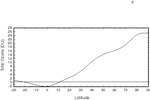
Figure 8. Anomalous total ozone during March, as a function of latitude, composited against total ozone at 50°N.
Anomalous total ozone in Figure 8 reflects interannual changes in the LS. Those changes are accompanied by interannual changes in the upper stratosphere. Lidar measurements at OHP, in addition to temperature, also retrieve ozone between 25 and 45km (Godin et al., 1985; Guirlet et al., 2000). Superposed in Figure 7 is the anomalous ozone column abundance above 30km observed at OHP (solid circles), after 1986. It misses a couple of years, due to limited sampling. Nevertheless, the available data from the upper stratosphere and mesosphere are strongly correlated to TOMS ozone fluctuations in the LS. In years when TOMS ozone is anomalously high, so too is OHP ozone. Just the reverse is observed in years when TOMS ozone is anomalously low.
Figure 9 shows the vertical structure of anomalous ozone mixing ratio at OHP (solid). Owing to the limited number of years available, March ozone has been composited by grouping high and low years and then differencing the means of each group. Anomalous mixing ratio is positive at all levels, decreasing upward from a maximum at 30km. Changes in the upper stratosphere thus operate coherently with changes in the LS, characterising ozone changes that are deep. When TOMS ozone (concentrated below 30km) is anomalously large, so too is ozone mixing ratio above 30km. Just the reverse is observed in years when TOMS ozone is anomalously small.
The structure of ozone changes above 30km mirrors the mean structure of ozone mixing ratio during March (dashed). Both peak near 30km and decrease upward in very similar fashion. The resemblance of anomalous ozone to mean ozone implies that much of the interannual change observed at OHP follows from a meridional swing of ozone mixing ratio surfaces: During winters when the residual circulation is strong, enriched mixing ratio surfaces expand poleward, as the vortex recedes. Conversely, during winters when the residual circulation is weak, those mixing ratio surfaces recede equatorward, as the vortex expands.
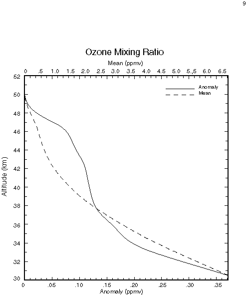
Figure 9. Anomalous ozone mixing ratio at OHP during March (solid), as a function of altitude, composited against ozone changes at 40km. Also shown is the 20-year mean ozone mixing ratio at OHP during March (dashed).
Observed changes of ozone in the LS have structure consistent with interannual changes of the residual circulation. So do contemporaneous changes of temperature. Interannual changes of ozone operating coherently in polar and tropical regions imply changes between neighbouring years (e.g., between ±1-2 std deviations of the residual circulation) of 50-100 DU. These are as large as observed changes that have been ascribed to chemical depletion.
Changes of temperature and ozone in the upper stratosphere and mesosphere operate coherently with changes in the LS. They evidence an expansion of ozone-rich air at subpolar latitudes during winters when the residual circulation is strong, compensated by reversed changes of ozone-lean air inside the polar vortex.
Changes of the residual circulation introduce changes of photochemistry, which can change ozone as well. Changes of meridional transport alter ozone production inside air that drifts poleward during the disturbed season. Such changes also influence chemical destruction mechanisms. Winters when the residual circulation is anomalously weak lead to temperatures over the Arctic that are anomalously cold. They provide conditions more favourable for heterogeneous processes, like those operating in the Antarctic LS. Conversely, winters when the residual circulation is anomalously strong lead to temperatures over the Arctic that are anomalously warm, making such processes unlikely.
Through this mechanism, interannual changes of the residual circulation can regulate ozone depletion over the Arctic. While heterogeneous chemistry can augment changes introduced directly by changes of transport, it's unlikely that it plays a central role in observed changes of temperature and ozone. Those interannual changes have structure that is deep, extending upward coherently through the entire stratosphere. They also operate coherently across much of the globe, changes at high latitudes being compensated at low latitudes by changes of opposite sign.
Baldwin, M., 2000: The Arctic oscillation and its role in stratosphere-troposphere coupling. SPARC Newsletter, 14, 10-14.
Fusco, A. and Salby, M.L., 1999: Interannual variations of total ozone and their relationship to variations of planetary wave activity. J. Climate 12, 1619.
Godin, S., G. Megie, and J. Pelon, 1989: Systematic Lidar Measurements of the Stratospheric Ozone Vertical Distribution, Geophys. Res. Lett., 16, 547-550.
Guirlet, M., P. Keckhut, S. Godin, and G. Megie, 2000: Description of long-term ozone data series obtained from different instrumental techniques at a single location: the Observatoire de Haute-Provence (43.9°N, 5.7°E). Annales Geophysicae (in press).
Hauchecorne, A., and M.-L. Chanin, 1980: Density and temperature profiles obtained by lidar between 35 and 70km. J. Geophys. Res. Lett., 7, 565-568.
Holton, J.R., and H.-C. Tan, 1980: The influence of the equatorial quasi-biennal oscillation on the global circulation at 50mb. J. Atmos. Sci., 37, 2200.
Keckhut, P., A. Hauchecorne, and M.-L. Chanin, 1995: Mid-latitude long-term variability of the middle atmosphere: Trends and cyclic and episodic changes. J. Geophys. Res. Lett., 100, 18, 887-18, 897.
Labitzke, K., 1982: On interannual variability of the middle stratosphere during northern winters. J. Meteorol. Soc. Japan, 60, 124.
Thompson, D. and J.M. Wallace, 1998: The Arctic oscillation signature in the wintertime geopotential height and temperature fields. Geophys. Res. Lett., 25, 1297.
Thompson, D. and J.M. Wallace, 2000: Annular modes in the extratropical circulation, Part II: Month-to-month variability. J. Climate, 13, 1018.
Tung, K.K. and H. Yang, 1994: The influence of the equatorial quasi-biennial oscillation on the global circulation at 50mb. J. Atmos. Sci., 51, 2708.
WMO, 1995: "Observed Changes in Ozone and Source Gases". WMO, Rep. No. 37.
WMO, 1999: "Scientific Assessment of Ozone Depletion: 1998". WMO, Rep. No. 44.
![]()