Figure 1: The atmospheric temperature profile (US Standard Atmosphere, 1976). To the four regions correspond very different temperature gradients.
Table of Contents
1. Structure and Composition of the Atmosphere
2. Chemistry of the Troposphere
2.1 Oxidizing Capacity
of the Troposphere
2.2 Formation of the OH
Radical
2.3 Oxidation of Methane
2.4 Oxidation of Carbon Monoxide
4. Tropospheric Carbon Monoxide
4.1 Budget
4.2 Spatial and Temporal
Variability
For study and reference, scientists have separated the atmosphere into four regions, very different in their structure, thermodynamics, photo-chemistry and dynamics. This partition is best reflected by the atmospheric vertical temperature profile, whose points of inflection are used to distinguish the four regions (Figure 1). Starting from the ground, they are called the ‘troposphere’, the ‘stratosphere’, the ‘mesosphere’ and the ‘thermosphere’, and the boundaries separating them the ‘tropopause’, the ‘stratopause’ and the ‘mesopause’.
The atmospheric thermal structure is ultimately defined by a combination of dynamic and radiative transfer processes. The troposphere is heated from the ground, which absorbs solar radiation and releases heat back up in the infrared. The temperature of the air in this region therefore decreases linearly with altitude, at a lapse rate of 5 to 7 K km-1, or a little over half a degree per 100 m, as common knowledge suggests. The tropopause, situated between 8 km (at high latitudes) and 15 km (at the equator), marks the end of this linear decrease and the beginning of the stratosphere, where lies the bulk of atmospheric ozone (the ‘ozone layer’). The presence of ozone is vital for life on Earth, as it absorbs the dangerous part of incoming ultra-violet radiation. As a result, the stratosphere heats up and has a positive temperature gradient. The temperature peaks at the stratopause at approximately 50 km in altitude, then falls linearly again in the mesosphere, as ozone heating diminishes. The region of the atmosphere above the mesopause is called the thermosphere and is radically different from the three lower regions. It cannot be treated as an electrically neutral medium because energetic solar radiation ionizes the molecules and atoms to form a plasma of free electrons and ions that interact with the Earth’s magnetic field.
Figure 1: The atmospheric temperature
profile (US Standard Atmosphere, 1976). To the four regions correspond very
different temperature gradients.
The word troposphere means ‘turning sphere’, which symbolizes the
fact that, in this region, convective processes dominate over radiative
processes. The troposphere is indeed marked by strong convective over-turnings,
whereby large parcels of warm air travel upwards to the tropopause, carrying
water vapor and forming clouds as they cool down (the stratosphere, on the
other hand is a very stable a stratified environment where heat transfer
is mainly radiative). The troposphere contains the bulk of atmospheric water
vapor, the majority of clouds and most of the weather, both on a global and
a local scale. Because pressure decreases exponentially with altitude, it
also contains over 75% of the total mass of the atmosphere. Most importantly,
however, it is in contact with the Earth’s surface and therefore interacts
directly with other climate subsystems, such as the biosphere (the land and
vegetation), the hydrosphere (the oceans), the cryosphere (the ice caps),
the lithosphere (the topography), and most all, with the human world (Peixoto
and Oort, 1992).
Table 1: The composition of the atmosphere (adapted from Salby, 1996). All values are mean tropospheric values.
The bulk of dry air is made up of nitrogen (78% by volume) and oxygen (21% by volume). Noble gases, carbon dioxide and a large number of other minor gases constitute the remaining 1% of the atmosphere. Although they are in very small concentrations, these trace constituents play a vital role in all aspects of atmospheric physics and chemistry (in contrast with nitrogen: inert and uninteresting). Table 1 gives the average tropospheric abundance of a selected number of species. Note that the gases of interest in this work, namely methane and carbon monoxide, have mixing ratios expressed in ppmv and ppbv. Most constituents are distributed fairly evenly up to the mesopause, with the exception of water vapor, which is mostly confined to the troposphere, and ozone which is concentrated in the stratosphere (Figure 2).
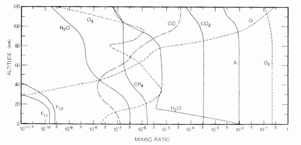
Figure 2: Vertical profiles of the mixing
ratios of selected species at the equinox (from Goody and Yung, 1989).
2. Chemistry of the troposphere
2.1 Oxidizing Capacity of the Troposphere
As mentioned above, nowhere around the Earth is the air perfectly clean: besides nitrogen, oxygen, inert gases, carbon dioxide and water vapor, it contains many trace pollutants. Be they emitted by natural or anthropogenic sources, they heavily influence our climate system. Natural sources include volcanoes eruptions, swamps, wild animal emissions, forest fires and dust, while anthropogenic ones include industrial activities, fossil fuel burning, car usage, emissions from domestic animals and agriculture. Because of its growing importance, the latter category is very publicized and becoming common knowledge even amongst the non-scientific community. Fortunately, the atmosphere has up to now avoided any substantial accumulation of pollutants, thanks to a remarkable natural ability to cleanse itself. There are three end removal processes. The first is chemical conversion to non-polluting constituents, such as H2O or O2. The second is dry deposition, whereby gases are absorbed by plants, water or soil. It is of limited significance because it often only applies to gases in the boundary layer on a local scale. The third is wet deposition, or removal by precipitation, and is only effective for species that have enough solubility in water, which is not the case in general. There are, however, a number of tropospheric species capable of oxidizing these pollutants so that they become soluble. Although these species are only present in minute amounts, they constitute the pivot of tropospheric chemistry.
Ironically, the discovery of the oxidizing capacity of the troposphere came relatively late and through indirect reasoning. In 1970, Pressman and Warneck noted that, although the emission of CO had been steadily increasing over the 50's and 60's, there was no repercussion on its tropospheric concentration. The puzzle was solved a year later when Levy (1971) found a route for the formation of OH radicals in the troposphere and suggested that they could be a major sink for CO. The importance of OH radicals and other oxidants as the detergents of the atmosphere has been recognized ever since. They are, in descending order of importance:
Together, these oxidants determine the lifetime and the abundance of trace
species, acting as a atmospheric regulators. The reverse is also true: the
abundance of trace species regulate the oxidizing capacity of the atmosphere,
since an increase in the emission of a given pollutant reduces the abundance
of its principal oxidant. The resulting positive feedback may even eventually
lead to an increase of other pollutants. This underlines the importance of
a stable oxidizing capacity in the troposphere, of prime importance to our
environment.
 |
 |
 |
Figure 3: Removal of OH by trace gases in the upper troposphere (adapted from Warneck, 1993). CO is the main sink, destroying over half of the total amount in all cases. Although CH4 comes next in order of importance, only destroying between 8 and 18% of OH radicals, it has a predominant role in the oxidation cycle (the cycle is often referred to as the methane oxidation cycle). The chemical processes leading to the destruction of OH are not straightforward because the radical may be re-cycled many times or yield other oxidants before it is finally destroyed. Incidentally, the rate of oxidation with a given pollutant depends on the mixing ratio of the pollutant, the reaction rate, the reaction efficiency and external conditions such as temperature and pressure.
Figure 4: Sinks of hydroxyl in the continental boundary layer.
Figure 5: Sinks of hydroxyl the marine boundary layer.
2.2 Formation of the OH radical
The basic ingredients for the formation of hydroxyl are NO and NO2, water vapor, ozone and radiation at wavelengths shorter than 315 nm: in simple terms, NO2 is very reactive and may form O3, which in turn may yield hydroxyl. NO2 is mainly created through oxidization of NO, itself an indirect product of biomass burning, high temperature combustion and microbial actions in the soil. It is thought that the first two man-made sources represent up to 50% of the total emissions.
The process for in-situ ozone production by NO2 can be written as
(Wayne, 1991). A similar reaction involving alkyls may be written down by replacing NO2 by RO2 in the above equations. Below a certain value of [NO]'[O3], it is worth noting that ozone is actually lost, because the destruction sequence dominates over the generation sequence. The destruction sequence has the net result
On average ozone maintains itself in the troposphere at levels between 25 and 30 ppbv. It may be photolysed at wavelengths around 310 nm to yield an exited O(1D) oxygen atom that reacts with water vapor to form two OH radicals (if not quenched back to its ground state through a collision with nitrogen or oxygen molecules):
It is should be pointed out that the quenching process does not constitute a loss of ozone because almost all ground state oxygen atoms react with oxygen to regenerate ozone with the help of a third body:
![]() (2)
(2)
2.3 Oxidation of methane
Depending on NOx levels, methane oxidation may either be a production or a destruction process for odd hydrogen. In general, high concentrations of nitrogen oxide are found in the polluted northern hemisphere or in boundary layer of the tropics, and low levels in the southern hemisphere. In regions of high levels of NOx, methane oxidation primarily occurs via the sequence
(H2) ![]() (2)
(2)
(H2) ![]() (1)
(1)
(Wubbles and Tamaresis, 1993). One of the final products is ozone, which feeds back into the creation of OH radicals, as discussed earlier. The second is formaldehyde (CH2O) which may be oxidized to form carbon dioxide. There are three different paths leading to the creation of CO, all involving NOx. The first is a simple photolysis:
The second also starts with photolysis but has different products, namely CHO and H. The resulting sequence of reactions gives the net product
The third pathway is initiated by a hydroxyl attack and gives the net product
The fractional contribution of the three equations are roughly 55%, 25% and 25% (Crutzen, 1988). They constitute together an important source of tropospheric carbon monoxide.
In regions of low NOx concentrations, the oxidation of methane takes two pathways, both initiated by a hydroxyl attack
![]() (11)
(11)
![]() (12)
(12)
followed by
or
(Wuebbles and Tamaresis, 1991). The branching ratio for the two pathways, according to DeMore (1990) is 70% to 30%. Both sequences yield two moles of water vapor per mole of methane. Besides, the first produces formaldehyde that is either washed out by wet deposition or is oxidized to carbon monoxide.
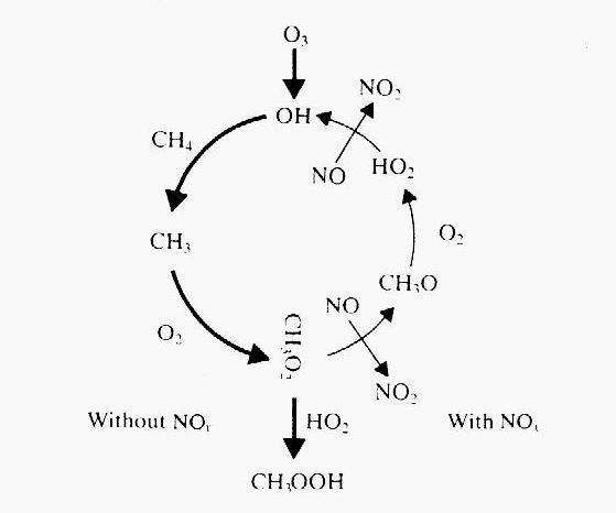
Figure 6: Schematic of the CH4 oxidation cycle
(from Wayne, 1991). The bold arrows in the first half of the cycle indicate
what happens without NOx, while the thin arrows on the second
half indicate processes that require NOx, and close the loop back
to the formation of hydroxyl.
In summary, NOx plays a very important role in the methane oxidation
cycle. If it is sufficiently abundant, it closes the loop of a
cycle that regenerates hydroxyl. In its absence, the cycle terminates abruptly
and methane becomes a sink for hydroxyl. This double role is schematically
represented in Figure 6.
Like the methane, the oxidation cycle of carbon monoxide depends on the level of NOx. In high NOx regions the oxidation sequence is
![]() (3)
(3)
![]() (4)
(4)
![]() (5)
(5)
Again, the transformation of NO into NO2 regenerates a mole of OH radicals for each mole consumed in the CO oxidation reaction, and there is no net loss of oxidants. In turn, NO2 may be photolysed to initiate the production of ozone and hydroxyl:
![]() (1)
(1)
![]() (2)
(2)
The net product of the last five equations can be written
![]() (6)
(6)
In unpolluted regions, the sequence is
![]() (3)
(3)
![]() (4)
(4)
![]() (7)
(7)
Regardless of the levels of NOx, both sequences generate carbon dioxide on a mole to mole basis. In polluted regions, the oxidation of CO generates (also on a mole to mole basis) ozone, a vital precursor to hydroxyl, an oxidant in its own right, as well as a potent greenhouse gas. In unpolluted regions, on the contrary, the oxidation of CO consumes ozone (Cicerone, 1988).
In conclusion, I wish to underline the fact that methane and carbon monoxide have arguably the most important roles in the hydroxyl oxidation cycle, itself the main scavenger in the troposphere. In fact, the simplified equation for OH concentration
where ki are reactions rates (in s-1) and [NMHC] is the concentration of non-methane hydrocarbons, is often accurate enough for many practical calculations (Wuebbles and Tamaresis, 1993).
Methane is well mixed over the entire globe, largely because its lifetime is about a year. Although the global average concentration of methane is slowly increasing, its emission rate is, to a first approximation, equal to the destruction rate at a level between 450 and 550 Tg yr-1. Sources of tropospheric methane fall into two categories (Figure 7). Anthropogenic sources constitute over 80% of the total methane production and include rice paddies, cattle enteric fermentation, gas drilling, coal mining, landfills and biomass burning. The natural sources of methane are wetlands, swamps, termites, lakes and oceans. The strength of these sources have been the subject of a heated debate over the last 20 years for the simple reason that it is extremely difficult to make reliable estimations. Consequently, the value for the total budget varies wildly from study to study. In addition, sources emitting less than 5 Tg yr-1 (urban areas sewage disposals, natural gas leakage and tundra) have not yet been studied in any depth and it is probable that more sources remain unidentified. Incidentally, the knowledge of their emission rates is not relevant for the budget calculation because major sources already have huge uncertainties associated to them.
Figure 7: A breakdown of the sources of
methane (adapted from Whiticar, 1993). Their relative and absolute strength
still give rise to controversy. Nonetheless, Whiticar’s estimate of
the total emission at x =540 Tg yr-1
agrees within reason with the work of Ehhalt (1974), Khalil and Rasmussen
(1983) and Crutzen (1983), who give respectively
533<x <854 Tg yr-1,
x =553 Tg
yr-1,170<x <620 Tg
yr-1.
A large part of the production of methane occurs in swamps, marshes rice paddies, shallow lakes and fermentation tanks of sewage disposals. Methanogenic bacteria belong to a group of anaerobes living in symbiosis with other bacteria that derive their living from cellulose and other organic material. These bacteria produce amongst other compounds CO2 and H, which are transformed by methanogens into methane. The gas escapes through the sediments and the water only if the depth does not exceed 10m, otherwise it is oxidized before reaching the open air.
Methane escapes from the surface of oceans because it is slightly supersaturated with respect to the boundary layer, due to the presence of anaerobic bacteria. Models for the diffusion process have been proposed but there is some degree of uncertainty associated with extracting an absolute value for the methane flux, because of variations in the film thickness and temperature and the agitation of the sea by the wind (Ehhalt, 1974; Seiler and Schmidt, 1974a).
Enteric fermentation occurs in the stomach of herbivores, most of which are domestic. Studies by Ehhalt (1974) show that out of a total of 45 Tg, cattle contributes up to 60%, horses to 30%, and sheep and goats to 5%. Methane is also produced by the digestion of herbivorous insects, such as termites, whose digestive tract host symbiotic microorganisms. The digestion of termite releases CO2 and methane in the ratio 0.0077, which yields a total around 50 Tg per year, but there has been controversy over this number (Warneck, 1988).
Other anthropogenic sources include emissions from coal and lignite mining fields, chemical and petroleum industries, car exhausts, gas-well leaks, combustion of agricultural wastes, forest fires and forest clearances for agricultural purposes (especially in the tropics). Biomass combustion, for example, yields a volume ratio of methane to carbon dioxide between 1 and 2.3%.
There are, on the other hand, only three relatively well known sinks for tropospheric methane: oxidation by OH radicals, loss to the stratosphere and soil uptake. Khalil et al. (1993) estimates that 440 Tg yr-1 of methane is destroyed in the troposphere by hydroxyl in the daytime and 5 Tg yr-1 in the night time. The bulk of the destruction occurs in the tropics and very little at higher latitudes (above 50B most of it takes place during the summer). Scavenging in the stratosphere by OH could account for 10 Tg yr-1, by O(1D) for 5 Tg yr-1 and by Cl for just over 1 Tg yr-1. Finally the total soil sink is estimated to be 25-30 Tg yr-1, yielding a total sink strength of around 490 Tg yr-1.
There is a general consensus that the average concentration of methane in the atmosphere is increasing at a current rate of nearly 1% per year in both hemispheres. It is essentially due to the dramatic increase in agricultural and industrial emissions coupled to global population growth. This rate was found to be rather constant over the last decade, a period over which measurements have become more reliable and spatially extensive. With the records extracted from bubbles of air trapped in polar-ice, there is even evidence that levels of CH4 have been steadily rising over the last 1000 years, with an twofold increase to the present value of 1.7 ppbv between the 18th century and nowadays. Older ice-core records also suggests that the concentration of methane has been very erratic over the last 160,000 years, with oscillations by factors of 2 on time scales of 10,000 years. These variations correlate extremely well with those of temperature and underline the importance of methane as a greenhouse gas (Raynaud and Chappellaz, 1993; Ehhalt, 1988).
The effect of increasing methane concentration on the oxidizing capacity of the atmosphere, and on hydroxyl levels in particular is very difficult to assess, due to the lack of convincing experimental data (Wuebbles and Tamaresis, 1993). Thompson et al. (1990) used a one-dimensional model to study the repercussion of methane and carbon monoxide increases on levels of ozone and hydroxyl for chemically coherent regions for the period between 1985 and 2035. He found that with an increase of 0.8% per year for methane and 0.5% for carbon monoxide, hydroxyl levels could fall by 15% in unpolluted regions, but only by a few percent in highly polluted urban areas. Any decrease of the concentration of hydroxyl, however, would initiate a positive feedback process that could ultimately lead to a sharp drop in the oxidizing capacity of the atmosphere and an accumulation of pollutants.
Although methane’s atmospheric abundance is less than 0.5% that of carbon dioxide, it is also a very important greenhouse gas: methane is in fact 20 times stronger. Its direct effect on radiative forcing is not to be underestimated: a twofold increase in methane concentration is predicted to generate a 0.42 W m-1 negative forcing (against 4 W m-1 for CO2). Indirect effects on climate include the production of CO2, water vapor (one mole produced for each mole of methane) and ozone, all major greenhouse gases. The overview by Wuebbles and Tamaresis (1993) details some of the research that has been carried out on this subject over the last ten years.
4. Tropospheric Carbon Monoxide
As for methane, the budget of carbon monoxide is difficult to determine precisely
and varies from source to source. In this light, I present in Figure 8 and
Figure 9, two separate studies, respectively by Logan et al. (1981) and Seiler
and Conrad (1987) and refer the reader to Warneck (1988) for a more complete
overview of the problem. Logan’s total CO source strength is estimated
to be 2736 Tg yr-1, out of which 1813 Tg yr-1 comes
from the northern hemisphere and 922 Tg yr-1 from the southern
hemisphere. Seiler, on the other hand, estimates this number to be 3300
± 1700 Tg yr-1, with the tropics
representing 1900 ± 1100 Tg yr-1.
Moreover, Logan calculates the total CO sink to be 3400 Tg yr-1
(i.e. larger than his source estimation) while Seiler calculates it to be
2500 ± 1700 Tg yr-1 (i.e. smaller
than his source estimation). Besides global source and sink strengths, the
breakdown of the budget into the individual sources is also plagued by large
uncertainties.
Figure 8: Sources
ans sinks of CO (adapted from Logan et al., 1981).
Figure 9: Sources ans sinks of CO (adapted from Seiler and Conrad
1987). The tropics encompass latitudes between
30° N and
30° S.
In the northern hemisphere, anthropogenic emissions are responsible for the bulk of CO emission, because 90% of the world population lives there. According to Logan, fossil fuel burning represents 14% of the total emission, emitting 450 Tg yr-1. In this category, automobile accounts for 52% of the emissions, industrial processes (especially the production of steel and the catalytic cracking of crude oil) roughly 29%, energy conversion 14% and waste disposal 5%.
Anthropogenic destruction of biomass represents some 850 Tg yr-1. In the tropics, this destruction is largely associated to agricultural practices such as slash, burn, shift and burning of grassland at the end of the dry period. In temperate climate zones, these practices are negligible but disposal of agricultural waste is important.
Oxidation of methane is another important source of CO (810 Tg yr-1), because carbon monoxide is an indirect product of the methane oxidation cycle: it created in polluted regions on a mole to mole basis through the photolysis of formaldehyde, which is itself a direct product of methane oxidation (section 2.3).
Oxidation of non-methane hydrocarbon (NMHC), on the other hand, only yield 90 Tg yr-1. Emissions from plants are the largest source of NMHC’s, principally in the form of isoprene and terpenes. The former are primarily issued from deciduous plants, notably oak, during daylight and the latter from conifers. A study by Zimmerman et al. (1978) found that terpene emission varied with temperature and therefore season and latitude and that the bulk of it occurred in the tropics. Zimmermann also suggested a global average ratio of hydrocarbon emission to the net primary productivity of 0.7%, which yields a isoprene and terpene emissions respectively of 350 Tg yr-1 and 480 Tg yr-1. The oxidation of isoprene is fairly well understood and produces CO and CO2 in the ratio 1/4. The CO yield of terpene oxidation is estimated by Hanst et al. (1980) at 20% but is more uncertain. These numbers suggest production rates from emissions from plants of 576 Tg yr-1 and 198 Tg yr-1 respectively for isoprene and terpene, totaling 774 Tg yr-1 somewhat larger than Logan’s estimation of 560 Tg yr-1. Note that green plants are also net producers of CO (130 Tg yr-1, according to Logan), through a mechanism that is still not clearly identified.
Finally, CO is released from the surface of oceans in the same way as methane: surface waters are believed to be slightly supersaturated with CO by a factor of 30± 20 and release between 70 and 220 Tg yr-1 (depending on the authors) fairly independently of latitude (Warneck, 1988). For his budget calculation, however, Logan retains the smaller value of 40 Tg yr-1.
The stratosphere as a sink for CO, identified in the late 1960’s, simply
arises because of the continuous gradient in CO concentration across the
tropopause and represents approximately 200 Tg yr-1 (Seiler and
Conrad, 1987). As for soils, they act as a sink when the steady-state CO
mixing ratio in the air above them is lower the that of ambient air and as
a source when it is higher. The steady-state value is highly dependant on
humidity, temperature, soil type and bacteria content, in such a way that
apart from arid areas, moist soils act as a sink. CO consumption in soils
is without any doubt due to bacteria, although the exact type of micro-organisms
involved is still uncertain. Warneck (1988) gives a brief review of the different
laboratory experiments and other studies on the subject and all converge
to a net sink strength between 200 and 600 Tg yr-1: Logan settles
on 250 Tg yr-1 and Seiler and Conrad on 495 Tg yr-1.
The main sink by far, however, is oxidation by hydroxyl which represents
between 80 and 95% of CO losses in the atmosphere.
4.2 Spatial and temporal variability
In the cities, CO mixing ratios are in the range 1-10 ppmv, due to emissions from automobiles mainly. In clean air regions of the northern hemisphere, levels fall to 200 ppbv and in those of the southern hemisphere to 50 ppbv on average (Figure 10). Studies since beginning of the 1970's have demonstrated the existence of this latitudinal gradient and shown that the transport of CO from the one hemisphere to the other occurs mainly in the upper troposphere (Figure 11).
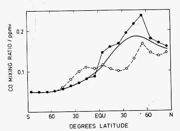
Figure 10: Latitudinal gradient of CO mixing ratios over the Atlantic Ocean
(adapted by Warneck (1988) from Seiler and Schmidt, 1974). The open circles
correspond to aircraft measurements in the upper troposphere at about 10
km in altitude, the filled circles to sea-level measurements onboard of ships
and the solid line to the mass-weighted average of the two.
Below 50B S, where anthropogenic sources are negligible, the concentration of CO reaches a photo-chemical stationary state, in which CH4 is its major source and OH is only sink. The concentration may then be approximated by
where ki are reaction rates and S2 is a secondary source of CO. The equation implies that CO levels are intricately dependant on OH levels and in this respect agrees fairly well with observation data (Figure 12): the abundance of CO hardly rises above 20 ppbv in the months of December to April, and exceeds 70 ppbv between May and November (in the meantime, the background level of OH is high in the summer and low in the winter, as a consequence of the variation in the solar radiation flux). Seiler calculates that OH accounts for 52% of the total CO source term and that the secondary source S2 must be seasonally independent. This is not the case of most known CO sources and it is therefore possible that there are several secondary contributors whose temporal variations cancel out. The main secondary source in the southern hemisphere is thought to be a ~160 Tg yearly flux of CO from the northern hemisphere, due to the difference in the mass content between the hemispheres (~310 Tg for the northern hemisphere and ~150 Tg for the southern hemisphere). In the tropics and the northern hemisphere, hydroxyl is also the main CO sink, but the presence of multiple sources renders its temporal variability more complex. The levels of CO depend critically on the seasonal cycles of human activities and natural processes outlined in the previous paragraph. Likewise, the spatial variations of CO are correlated to variations in the human activity and the biomass.
The mean residence time of CO in the atmosphere, t CO, can be estimated from its total budget figure and average concentration. The global budget estimate of Seiler and Conrad (1987) gives t CO = 2 months while that of Logan et al. (1981) gives t CO = 2.5 months. This essentially means that the burden of CO in the atmosphere is on average completely replaced 6 times per year, not leaving enough time for CO to get evenly mixed around the globe. In is important to realize, however, that t CO is not singled valued: this would mean that sources and sinks have the same temporal and spatial variations, which is not the case. For example, the levels of OH are much larger in the boundary layer than in the upper troposphere and in the summer than in the winter. Thus CO is much shorter lived in the boundary layer during the summer than in the upper troposphere during the winter.
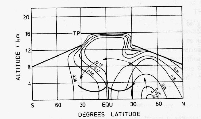
Figure 11: Longitudinal cross-section
of the vertical transport of CO over the Atlantic Ocean (adapted by Warneck
(1988) from Seiler and Schmidt, 1974). The contours give the mixing ratios
of CO in ppmv and the arrows materialize the CO flux from the northern to
the southern hemisphere.
In the 1970’s and 1980’s, measurements have suggested that the average concentration of carbon monoxide was rising at a rate of 1% yr-1 or higher. Graedel and McRae (1980), combining in-situ sampling and infrared absorption techniques from a large data set in New-Jersey (a highly polluted region), concluded to a small positive trend in the period between 1968 and 1977. Dvoryashina et al. (1984) measured the total column of CO between 1970 and 1982 and found a 1.7% increase for wintertime amounts and a 1.4% increase for summer amounts. The data, however, is biased towards high CO concentrations because measurements were made in clear skies only, synonymous of high-pressure conditions favoring the accumulation of anthropogenic pollutants. Khalil and Rasmussen (1984) reported the largest increase in that period (about 6% per year during 1979-1983), using gas chromatography in Oregon. A more complete review of 1960-1980’s measurements was written by Cicerone in 1988. In the recent years, however, studies have shown that this trend has been reversed. Khalil and Rasmussen (1994) find that the concentration of CO has decreased by 2.6% yr-1 between 1988 and 1992. Similarly, Novelli et al. found a drop of 6.1% in the northern hemisphere and 7% in the southern hemisphere from June 1990 to June 1993.
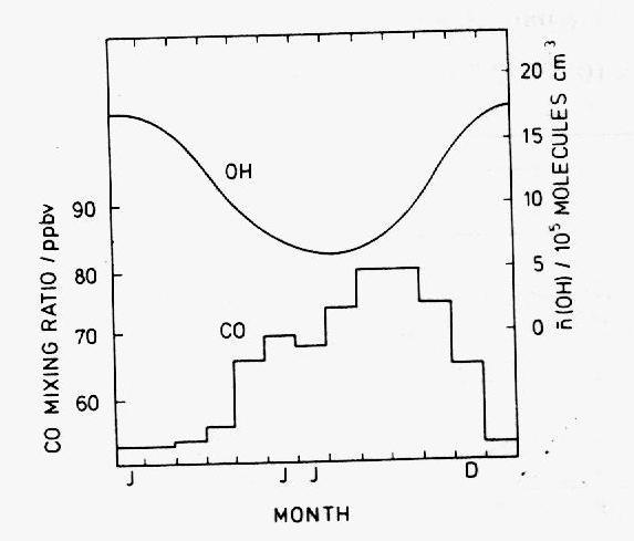
Figure 12: Monthly mean of the CO mixing ratio at Cape Point, South Africa
(34° S) averaged over the period 1978-1981
observed by Seiler et al. (1984) and OH number density calculated by Logan
et al. (1981).
M. Allen, Y.L. Yung and J.W. Waters, "Vertical Transport and Photochemistry in the Terrestrial Mesosphere and Lower Thermosphere (50-120 km)", J. Geophys. Res., 86, 3617, 1981.
M. Allen, J.I. Lunine and Y.L. Yung, "The vertical Distribution of Ozone in Mesosphere and Lower Thermosphere", J. Geophys. Res., 89, 4841, 1984.
R.J. Cicerone, "How has the Atmospheric Concentration of CO changed", The Changing Atmosphere, Edited by F.S. Rowland and I.S.A. Isaksen (Wiley), 49-61, 1988.
P.J. Crutzen and A.T. Gidel, "A Two-Dimensional Photo-Chemical Model of the Atmosphere: 2. The Tropospheric Budgets of the Antropogenic Chlorocarbons, CO, CH4, CH3Cl, and the Effects of various NOx Sources on Tropospheric Ozone", J. Geophys. Res., 88, 6641-661, 1983.
P.J. Crutzen, "Tropospheric Ozone: An overview", Tropospheric Ozone: Regional and Global Scale Interactions, Edited by I.S.A. Isaksen (D. Reidel, Boston), 3-11, 1988.
W.B. DeMore, S.P. Sander, D.M. Golden, M.J. Molina, R.F. Hampson, M.J. Kurylo, C.J. Howard, A.R. Ravishankara, "Chemical Kinetics and Photochemical Data for use in Stratospheric Modeling", JPL NASA Jet Propulsion Laboratory, 90-1, 47-48, 1990.
E.V. Dvoryashina, V.I. Dianov-Klokov and L.N. Yurganov, "Variations of the Content of Carbon Monoxide in the Atmosphere in the Period from 1970 to 1982", Izvestiya, 20, 27-33, 1984.
D.H. Ehhalt, AThe atmospheric Cycle of Methane", Tellus, 26, 1974.
D.H. Ehhalt, "How Has the Atmospheric Concentration of Methane Changed?", The Changing Atmosphere, Edited by F.S. Rowland and I.S.A. Isaksen (Wiley), 25-32, 1988.
R. M. Goody and Y.L. Yung, Atmospheric Radiation, Theoretical Basis, OUP, 1989.
T.E. Graedel and J.E. McRae, "On the Possible Increase in the Concentration of Atmospheric Methane and Carbon Monoxide during the Last Decade", Geophys. Res. Lett., 7, 977-979, 1980.
P.L. Hanst, J.W. Spence and O. Edney, "Carbon Monoxide Production in Oxidation of Organic Molecules in the Air", Atmos. Env., 14, 1220-1226, 1980.
M.A.K. Khalil and R.A. Rasmussen, "Sources, Sinks and Seasonal Cycles of Atmospheric Methane", J. Geophys. Res., 88, 5131-5144, 1983.
M.A.K. Khalil and R.A. Rasmussen, "Carbon Monoxide in the Earth’s Atmosphere: Increasing Trend", Science, 224, 54-56, 1984.
M.A.K. Khalil and R.A. Rasmussen, "Global Decrease in Atmospheric Carbon Monoxide Concentration", Nature, 370, 629-641, 1994.
M.A.K. Khalil and M.J. Shearer, "Sources of Methane: An Overview", Atmospheric Methane, Sources, Sinks and Role in Global Change, Edited by M.A.K. Khalil (Springer-Verlag), 1993.
M.A.K. Khalil, M.J. Shearer and R.A. Rasmussen, "Methane sinks and distribution", Atmospheric Methane, Sources, Sinks and Role in Global Change, Edited by M.A.K. Khalil (Springer-Verlag), 1993.
H. Levy, "Normal Atmosphere: Large Radical and Formaldehyde Predicted", Science, 173, 141-143, 1971.
J.A. Logan, M.J. Prather, F.C Wofsy and M.B. McElroy, "Tropospheric Chemistry: A Global Perspective", J. Geophys. Res., 86, 7210-7254, 1981.
R.E. Novelli, K.A. Masarie, P.P. Tans and P.M. Lang, "Recent Changes in Atmospheric Carbon Monoxide", Science, 263, 1587-1590, 1994.
J.P. Peixoto and A.H. Oort, "Chapter 2: Nature of the Problem", Physics of Climate, AIP, 8-26, 1992.
J. Pressman and P. Warneck, "The Stratosphere as a Chemical Sink for Carbon Monoxide", J. Atmos. Sci, 27, 155-163, 1970.
D. Raynaud and J. Chappellaz, "The Record of Atmospheric Methane", Atmospheric Methane, Sources, Sinks and Role in Global Change, Edited by M.A.K. Khalil (Springer-Verlag), 1993.
H.G. Reichle et al., "Middle and Upper Tropospheric Carbon Monoxide Mixing Ratios as Measured by Satellite-Borne Remote Sensor During November 1981", J. Geophys. Res., 91, 10865-10887, 1986.
H.G. Reichle et al., "The Distribution of Tropospheric Carbon Monoxide During Early October 1984", J. Geophys. Res., 95, 9845-9856, 1990.
M.L. Salby, Fundamentals of Atmospheric Physics, Academic Press, 1996.
W. Seiler and R. Conrad, "Contribution of Tropical Systems to the Global Budget of Trace Gases, especially CH4, H2, CO and N2O", The Geophysiology of Amazionia, Edited by R.E. Dickenson (Wiley, New-York), 133-160, 1987.
W. Seiler and U. Schmidt, "Dissolved Nonconservative gases in seawater", The Sea, Edited by P. Goldberg (Wiley New-York), 5, 219-243, 1974a.
W. Seiler and U. Schmidt, "New Aspects on CO and H2 Cycles in the Atmosphere", Proc. Int. Conf. Structure, Composition, General Circulation Upper Lower Atmos., Melbourne, 1, 192-222, 1974b.
W. Seiler H. Giehl, E.G. Brunke and E.A Halliday, " The Seasonality of Co Concentration in the Southern Hemisphere", Tellus, 36B, 219-231, 1984.
A.M. Thompson, M.A. Huntley and R.W. Stewart, "Perturbations of Tropospheric Oxidants, 1985-2035: 1. Calculations of Ozone and OH in Chemically Coherent Regions", J. Geophys. Res., 95-9, 829-844, 1990.
US Standard Atmosphere, Publication NOAA-S/T76-1562, Washington DC: US Government Printing Office, 1976.
J. Wang, J. Gille, P. Bailey, M. Smith, L. Liwen Pan, D. Edwards, L. Rokke, J.R. Drummond, G.R. Davis, H. Reichle, Measurement of Pollution in The Troposphere (MOPITT) Data Validation Plan, 1996.
P. Warneck, "Chapter 4: Chemistry of the Troposphere: the Methane Oxidation Cycle", Chemistry of the Natural Atmosphere, San Diego Academic Press, 131-175, 1988.
P. Wayne, "Chapter 5: The Earth’s Troposphere", Chemistry of Atmospheres, An Introduction to the Chemistry of Atmospheres of Earth, the Planets and their Satellites, Oxford Clarendon Press, 209-275, 1991.
D.J. Wuebbles and J.S. Tamaresis, "The Role of Methane in the Global Environment", Atmospheric Methane: Sources, Sinks and Role in Global Change, Edited by M.A.K. Khalil (Springer-Verlag), 469-513, 1993.
P.R. Zimmerman, R.B. Chatfield, J. Fishman, P.J. Crutzen and P.L. Hanst, "Estimates of the Production of CO and H2 from the Oxidation of Hydrocarbon Emissions from Vegetation", Geophys. Res. Lett., 5, 679-682, 1978.
 (24)
(24)
 (25)
(25)