Follow the directions from the guide sheet provided at the test.

Getting things up and running

The frequency generator: make sure that all buttons are not pressed, except for the "square wave" and "200Hz" range buttons. Choose a frequency of about 70-100Hz.
Set the knobs in a middle position and turn the " amplitude" knob to the maximum (extreme right)

Note: for some reasons, it may happen that a noisy picture gets less noisy if you turn down (say, at 1/2) the amplitude - your case may be different, but keep in mind that max. amplitude is not always the best choice in this experiment.

Connecting the wires:
from the generator apply the signal to the (left) driver;
monitor the signal applied to the driver on the channel A of the oscilloscope (pay attention to polarity: red to red, black to black!)
Signal from the pickup transducer is to be monitored on the B channel.

The oscilloscope:
Follow the directions from the Lab. Manual (the regular version of this experiment: read it now!).

Note: It's tricky to get a stable and clean picture on the screen. Keep Y_A and AUTO buttons pushed, play a bit with the "LEVEL" knob and see if it helps. Press and upress A button (switching on and off the reference signal display). Practice :-)

Take care: the inner knob (the fine-tuning little switch) on the time base [which controls the horizontal amplitude ] of the oscilloscope should be set in the "calibration" position (turn it to the extreme right until you hear a click).
Only this way you can trust the figures for the time conversion factors (time units/cm) on the big knob, and correctly get time measurements from the screen.

The write-up

Draw a diagram of the signal that you are measuring (a " screenshot ").
Clearly indicate the position of the square-wave applied to the driver and the signal received by the pickup transducer.
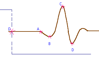
You have to measure the time delay corresponding to the OA segment. See my sketch below.

Take 5 - 6 data points (d,t), for different positions of the pick-up along the rod. Plot them on a d vs. t graph.
The guide sheet advises you to consider a 5% relative error in the time values. Please do as they ask :-) ; this way the error bars for the t axis should be visible pretty well.

As you probably observed, the fit line does not cross the origin (0,0) on the d vs. t graph.
This is a bit of surprise. Most probably we get this effect because of an unaccounted length in between the driver and the 0th mark on the measuring tape and also (presumably) some time delays in the transducer and/or driver. Both these are systematic errors (see Note 1 for a fix to this issue).
Nevertheless, the points should fit nice along a straight line and the slope of the fit line is the velocity of sound c  in the rod.

Note 1: To get a graph which passes through (0,0), you may try to plot (d_k -d₁) vs. (t_k -t₁).
Here d_k and t_k are the distance (time) of the k-th trial (k =1..N)
By construction, the new fit line should go through (0,0).
The advantage of this method is that it eliminates the errors due to the (unmeasurable directly) rod's length beyond the 0cm mark, and some possible time delays in the transducer a.s.o. Please, make sure you understand why this is so.

Note 2: On the other hand this trick makes your life complicated. In fact it is unnecessary, since the slope is the same! So, for the lab. test at least, there is no need to go through this tedious analysis.

The graph

Try to get a nice, large enough graph.
You'd probably have no error bars for the distance, but the error bars should be visible for the time (5% relative error, as suggested in the guide sheet).

Note 3: I'd expect to see a range of ( 0...70 )cm for the distance readings;
for the time range I would expect ( 0 ... 8 ) ms. See which are your values :-)
I found that for a frequency of f = (80.00 ± 0.05)Hz (or ± 0.1, if you like) the appropriate time basis is 0.1 ms/cm. During the preliminary setup you'll probably start with 1 ms/cm or 0.5 ms/cm scales, but you go to 0.1 ms/cm for the real measurements.
For the largest d of about 60cm, the useful signal ( OA ) extends on the whole screen (approx. 8-10 cm) while for d of about 20cm you still can see the signal comfortably (OA it's about 3cm) without moving to 0.05 ms/cm.

Write down the slope calculation on the graph and in your write-up.
Put the units wherever they need to be.

The error calculus

Use the method of minimal and maximal slope fit lines to get the error in the velocity of sound in the rod.
See the Lab. Manual (pp. 133-140) for details on how this method works.
Your min. and max. slope fit lines should look like the dash lines on this plot of d vs. t. At the lab. test your error bars will be different (because they are 5% of the t, not constants, as on my plot).

  Last revised: April 10, 2003
© Sorin Codoban 2003

Back to main page