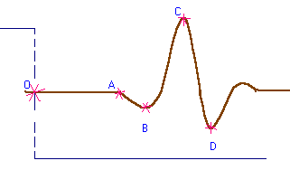
In the figure above you can see a sketch of what you (hopefully) get on
the screen of the oscilloscope as the signal received by the transducer.
By changing the position of the transducer on the rod, you may observe
that the features A, B, C, D move further right (as you increase the
the distance d - measured from the left driver).
To get the (d,t) plot you have to measure the time delay
OA (or OB, OC, OD) for each trial (i.e. different positions of the
transducer along the rod).
Is there a change in the slope of the fit line (i.e. in the velocity
retrieved from the graph) when using OB (or OC, OD) instead of OA? Why?
As you probably observed, the fit line does not cross the origin (0,0) on the (d,t) plot. This is a bit unexpected... Why?
To fix this problem, you may try to plot
dk -d1 versus tk
-t1. Here dk and tk
are the distance (time) of the k-th trial (k =1..N)
By definition, the new fit line should go through (0,0).
What about the slope?
Does it change (when compared with the initial plot)?
One of the advantages of this method is that it eliminates the
errors due to the (unmeasurable directly) rod's start length and
possible time delays in the transducer a.s.o.
Please, make sure you understand why this is so.
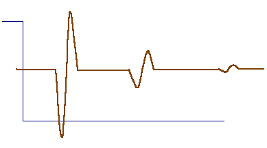
The plot above is a sketch of a screen shot (seen on the oscilloscope).
You may see this sort of image by applying the signal received at the
right-end
driver to the B-input of the oscilloscope (the A-input monitors the
signal applied to the left-end driver).
Note: it seems pretty dificult to get the
above image - at least in my experience only 1 of the 4 oscilloscopes
had the noise level low enough to get the above picture clearly. So, as
they say, your mileage may vary...Shop around for a better setup :-)
The spikes you see are consequently the first, the second, and the third
arrival of the wave at the end of the rod (due to repetead reflections).
The distance between the
first (counting from the left) to the second, and from the second to the
third spike corresponds to
the time of travel of the sound wave of
twice the lenght of the rod.
Obviously, one can use this setup to measure the speed of the sound in
the rod. Try this method, and compare the result with the
one obtained with the 'classic setup'.
Are you suprised by the result?
Possible explanations (= nice issue for the disscussion part of the
write-up)?
Last revised: May 22, 2003
© 2003, Sorin Codoban