We perform cubic and square fits with the data of the free fall of the plastic ball.
The difference between the fits is given by the errors in s and t . A table summarizing the results is provided at the end.
Note: the propagation of the errors is done by combining the
calibration error in s
with the reading error in quadratures. While this is
wrong in principle (calibration and reading errors have different
statistics - one is systematic, the other one is random error) the
effect of this wrong-doing is not that big. It works!
The correct approach would be
to take the reading error of
s to be the total error - for low
values of s. For large enough
values of s, the calibration error
(guide sheets say it is s/4000 )
is bigger than the reading error, so you take the calibration error
as your total error in s.
As a final note: combining the calibration and readings errors
as I did might be not that wrong in this case for a good reason.
Imagine that the calibration
error is generated by a "random" stretching/squeezing of
the meter tape during the manufacturing process. So, some regions of
the tape are shorter than those of a "right"
tape, while others are longer.
Since we don't know a priori what portions of the tape
are stretched / squeezed (and assuming that the
lengthscale of the anomalies is short enough - say, 10cm or so),
the expectation is that the calibration
error works as a random error in this case. Hence, the quadrature
combination of the two.
s (± Sqrt[2*(0.3)2+(s/4000)2] mm) vs. t (± 0.1 ms)
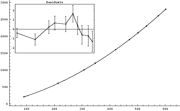 |
g2fit-1.gif (1-2)
v0 = (1.8068 ± 0.0026) m/s
( |
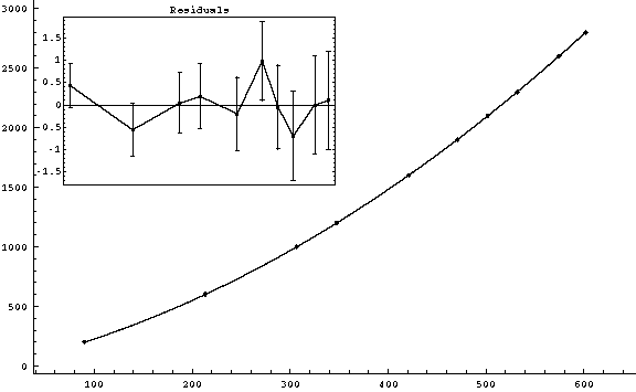 |
g3fit-1.gif (1-3) v0 = (1.7902 ± 0.0066) m/s
( |
s ( ± Sqrt[2*(0.3)2+(s/4000)2] mm) vs. t ( 0.05 ms)
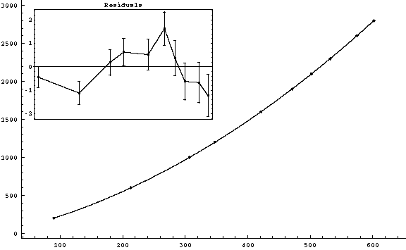 |
g2fit-2.gif (2-2)
v0 = (1.8071 ± 0.0022) m/s
( |
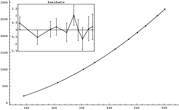 |
g3fit-2.gif (2-3) v0 = (1.7896 ± 0.0056) m/s
( |
s ( ± Sqrt[2*(0.2)2+(s/4000)2] mm) vs. t ( ± 0.05ms)
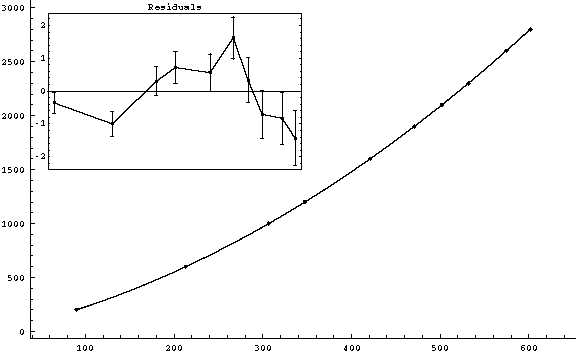 |
g2fit-3.gif (3-2)
v0 = (1.8060 ± 0.0018) m/s
( |
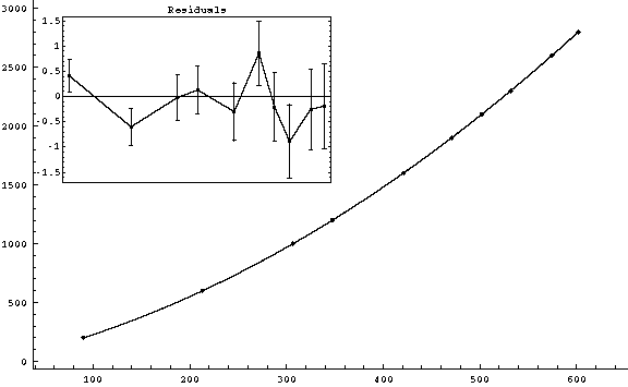 |
g3fit-3.gif (3-3)
v0
= (1.7905 ± 0.0043)
m/s
( |
s ( ± Sqrt[2*(0.2)2] mm) vs. t ( ± 0.05ms)
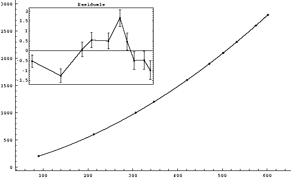 |
g2fit-4.gif (4-2)
v0
= (1.8083 ± 0.0014) m/s
|
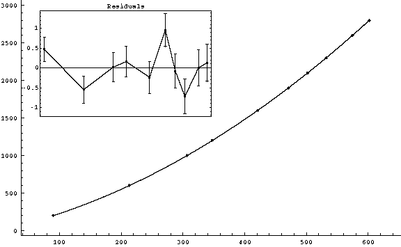 |
g3fit-4.gif (4-3) v0 = (1.7895 ± 0.0037) m/s
( |
s ( ± Sqrt[2*(0.3)2] mm) vs. t ( ± 0.05 ms)
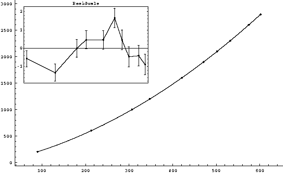 |
g2fit-5.gif (5-2)
v0 = (1.809 ± 0.0018) m/s
( |
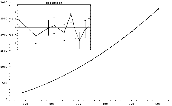 |
g3fit-5.gif (5-3)
v0 = (1.789 ± 0.005) m/s
( |
s ( ± Sqrt[2*(0.3)2] mm) vs. t ( ± 0.1 ms)
 |
g2fit-6.gif (6-2)
v0 = (1.8078 ± 0.0024) m/s
(
|
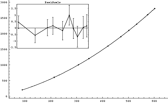 |
g3fit-6.gif (6-3)
v0 = (1.7899 ± 0.0062) m/s
( |
To summarize, we display below the main results from the above plots (rounded to significant digits)
|
Plot # |
v0 (m /s) |
g (m/s2) |
(m-1) x 103 |
reading s (mm) |
err. in t (ms) |
/ d.o.f. |
| 1-2 |
1.807 ± 0.003
|
9.465 ± 0.011
|
-
|
0.4
|
0.1
|
23.7 for 8
|
| 1-3 |
1.790 ± 0.007
|
9.70 ± 0.09
|
19 ± 7
|
0.4
|
0.1
|
3.53 for 7 .
|
| 2-2 |
1.807 ± 0.002
|
9.464 ± 0.009
|
-
|
0.4
|
0.05
|
16.8 for 8
|
| 2-3 |
1.790 ± 0.006
|
9.71 ± 0.06
|
19.6 ± 5.7
|
0.4
|
0.05
|
5.23 for 7
|
| 3-2 |
1.806 ± 0.002
|
9.469 ± 0.008
|
-
|
0.3
|
0.05
|
23.7 for 8
|
| 3-3 |
1.790 ± 0.004
|
9.70 ± 0.03
|
18.6 ± 4.7
|
0.3
|
0.05
|
7.84 for 7
|
| 4-2 |
1.8083 ± 0.0014
|
9.458 ± 0.006
|
-
|
0.3*
|
0.05
|
43.1 for 8
|
| 4-3 |
1.790 ± 0.004
|
9.715 ± 0.038
|
19.8 ± 3.7
|
0.3*
|
0.05
|
13.2 for 7
|
| 5-2 |
1.809 ± 0.002
|
9.456 ±0.007
|
-
|
0.4*
|
0.05
|
25.8 for 8
|
| 5-3 |
1.789 ± 0.005
|
9.72 ± 0.05
|
20 ± 5
|
0.4*
|
0.05
|
7.92 for 7
|
| 6-2 |
1.8078 ± 0.0024
|
9.46 ± 0.01
|
-
|
0.4*
|
0.1
|
14.2 for 8
|
| 6-3 |
1.790 ± 0.006
|
9.71 ± 0.06
|
19.5 ± 6.3
|
0.4*
|
0.1
|
4.39 for 7
|
* in those cases the error in s doesn't account for the (s/4000) calibration error. See the plots for details on error calculus!
Moral:
The value of g retrieved with a square fit
(frictionless theory) is typically (9.46 ± 0.01) m/s2.
It is
definitely far from the real value (g = 9.80m/s2, in MP building).
It looks like
the square fit is not a good choice; this is also pointed out by the  values
(typically 15...25 for 8 d.o.f.).
We can see a clear improvement in the case of a cubic fit (theory with friction).
The value retrieved is typically g = (9.71
± 0.06) m/s2 which, in the 2-sigma interval, "catches" the
precisely measured g (= 9.80 m/s2).
 values are typically 4...8
for 7 d.o.f., which also shows that the cubic fit is a good choice.
© Sorin Codoban, 2003.
 = ( 19 ± 7 ) 10-3 m-1