This page displays a few plots, done with Faraday's fit program.
The input is real data - for the plastic ball.These plots are similar to the plot you are supposed to draw by hand during the Lab. Test (shortly: LabT) for the "Free fall" experiment. The main purpose I pursue with this "plot show" is to give you a feeling of what kind of values you may expect to get during the real test, how the errors in s and t show up on the plot and in general, to give you an overview of what you can do yourselves, with your own data. Take advantage of the handy fit program and play a bit! It's a real pleasure .....
I must confess: I really hope that this page will not stop your desire to repeat and/or to go further in getting an insight on the Free Fall and others experiments. Let me know if this document acts as inhibition factor ...
Preliminaries
Data are analysed with the fit program, using the same formulae as at the LabT.
Namely, we try to see how well the frictionless theory describe the motion of the falling plastic ball. As at the LabT, we first derive a formula suitable for hand-made plot.
We start with s = v0 * t + (g/2)* t 2.
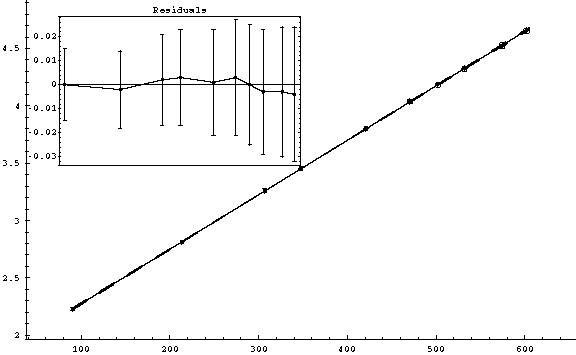
By dividing both sides by t one obtains s/t = v0 + (g/2) *t.Now, by plotting s/t vs. t you can easily see that the slope of the graph is just g/2.
As a byproduct we are also able to retrieve a value for the initial velocity v0 (as the intersection with the vertical axis).The plots below show you what values you'll get for g, under different assumption on the errors. Although you won't be able to do this kind of full error calculus, nevertheless I believe it would be helpful for developing a good intuition of numbers.
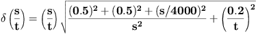
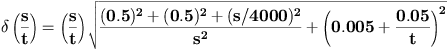
Note: I accounted for the calibration (accuracy) error ( which is s/4000 ) in an arguable manner. Namely, I combined it in qudratures with the random reading error for s. This is what Prep. Question no. 2 suggests, although in principle this is not correct (since the random and systematic errors cannot be combined in the same way - they have different behaviour).
On the other hand, the effect of this "wrongdoing" is not crucial for the conclusion of our experiment. If you have the time and will power, you may try to play around with different recipes for the error part of the analysis. One way of doing the error treatment better is to take as your error in s the bigger of the two (reading error vs. calibration s/4000).
Results:
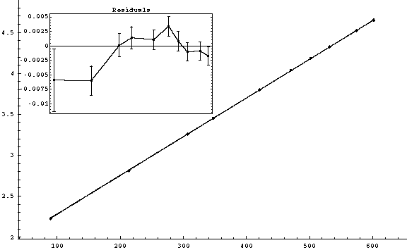
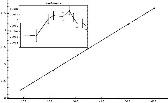
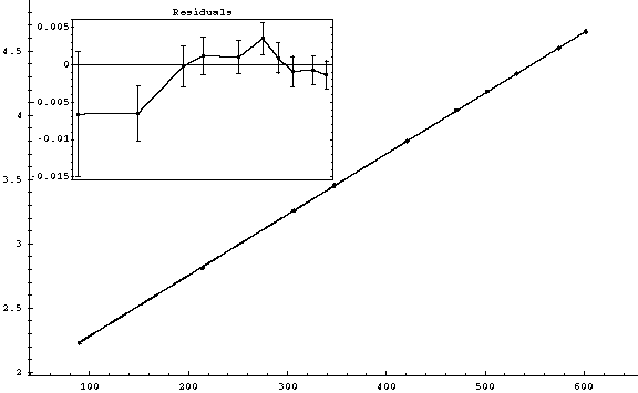
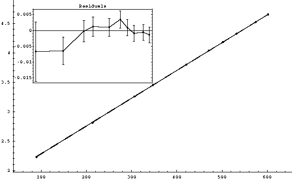
On all plots, on the vertical axis s/t (in mm/ms) is plotted.
On the horizontal axis t (in ms) is plotted.I quoted under each plot the formula used for the error calculation and the values for v0 and g retrieved from that graph.
The results are displayed in SI units ( m/s for velocity, m/s2 for acceleration).As a hint of how "good" the plot is, the
is also displayed. A plot is considered to be "good" when
(1)
Error in s/t (mm/ms):

Erorr in t (ms): 0.1
v0 = (1.8084 ± 0.0035) m/s
g = (9.458 ± 0.015) m/s2
(2)
Error in s/t (mm/ms)

Error in t (ms): 0.1
v0 = (1.8076 ± 0.0034)m/s
g = (9.460 ± 0.013) m/s2
(3)

Error in s/t (mm/ms):
Error in t (ms) : 0.05
v0 = (1.8069 ± 0.0033) m/s
g = (9.465± 0.007) m/s2
(4)
Error in s/t (mm/ms):
Error in t (ms): 0.05
v0 = (1.808 ± 0.0035) m/s
g = (9.46 ± 0.01) m/s2
(5)
Error in s/t (mm/ms):
Error in t (ms) : 0.1
v0 = (1.8093 ± 0.0045) m/s
g = (9.454 ± 0.015) m/s2
Note: if we were to pay attention only to
(6)
Error in s/t (mm/ms):
Error in t (ms): 0.2
v0 = (1.8094 ± 0.0062) m/s
g = (9.454 ± 0.015) m/s2
(7)
Error in s/t (mm/ms) :
Error in t (ms): (0.005*t+0.05)
v0 = (1.800 ± 0.013) m/s
g = (9.49 ± 0.08) m/s2
Note: This last plot illustrates a rather extreme assumption: the timer is supposed to have a 0.5% accuracy error, and this is accounted for in the same manner as we do it for multimeter measurements ( 0.5% + 1/2 digit ) - not quite the same expression, but the same idea.
Apart from an expected increase in the error for g it is nothing special here :-) ... Unless you are amazed by the 99.99% in
Read more about the meaning ofConclusion
There are a few interesting things one can learn from the above plots.
First, the mean value for g is constantly less than expected. Typically it's 9.45 ... 9.48 m/s2 with errors of 0.02 m/s2 or such. Even for a "good fit" like (5), g is far away from the expected 9.80 m/s2 value. Observe that I say "far away" because the 9.80 m/s2 is neither in a 1-sigma, nor 2-sigma distance from the mean value of g we got from the experiment.
Secondly, in all cases displayed above, the experimental points were lying on a straight line pretty well. You cannot see any spread in the points location. The residuals (in the rectangular frame on each plot) show you the region around the best fit line, zoomed-in - so you see how points lay around the line of best bit! But for a hand-made graph you shouldn't expect to see any deviation from that line, given the scale you may have for the plot.
Third, the error bars are too small to be displayed (in all cases - except for plot (7) where the errors are overestimated).
This means that you cannot apply the swinging/shifting of the fit line through the points in order to get an estimate of the errors in the slope from the graph. See Lab. manual (pag. 136) for details on how this procedure is supposed to work.The fit is a straight line as expected, but the value of g is consistently smaller than the known value (9.80 m/s2 ). This points out to the fact that the acceleration of the plastic ball is smaller due to some other effects, most probably because of the friction.
There is a catch here though, since friction depends on the velocity, and therefore the acceleration is not constant. Hence, using the frictionless theory (which assumes constant acceleration) to get the acceleration with friction it's not appropriate in principle.What can we do if we would like to get some estimate for the error in g ?
It's clear that even in the ideal case (of a nice spread around the line, and not a perfect alignment as we got it) we do not get by hand a value of error for g so precise as the fit program gives it. Perhaps we get it bigger, say by a factor of 2 or 3. This is a reasonable expectation.
As for our situation we are still "out of luck", because we cannot do the swinging/shifting required for error evaluation from the graph.So how do we get an error, anyway?
I have some clues about what can be done ...Hint: try to draw the graph by hand and see how accurately you are able to:
a) put the points in their places,
Hint question:
are you able to plot the values of t and s/t given with 4 significant digits?b) draw the "exact" line of best fit,
c) read the raise and run of the line right from the graph, to calculate the slope.
Well, I guess you already figured it out that the situation is far for being desperate. There are plotting and reading-from-the-graph errors in all the steps above!
You just have to account for them and get the error in g.Back to main page
Last updated: April 7, 2003
© Sorin Codoban, 2003.