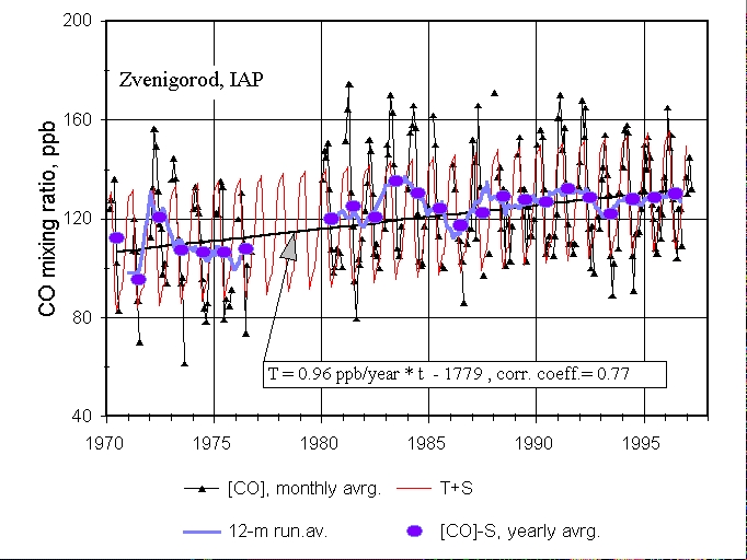
Figure 1. Total column CO abundance over Zvenigorod, Russia, presented as weighted mean mixing ratio ([CO]) for the tropospheric depth. In the box is linear trend T(t), S is the seasonal cycle (see text).
Zvenigorod Carbon Monoxide Total Column Time Series:
27 Years of Measurements
L. N. Yurganov
Department of Physics, University of Toronto, Toronto, Ontario M5S 1A7,
Canada; e-mail leonid@atmosp.physics.utotonto.ca
E. I. Grechko and A. V. Dzhola
Institute of Atmospheric Physics, Russian Academy of Sciences, Moscow,
109017, Russia
Abstract
The analysis of total column spectroscopic CO observations over Russia
between 1970 and 1996 revealed an upward trend, with a rate of 0.96 ppb/year
or 0.9 %/year. A similar trend has been reported over Switzerland between
1950 and 1987. This rate of CO growth is almost 3 times higher than the
rate between 1920 and 1950, obtained from ice core data. However, after
1982, CO above Zvenigorod varied from year to year with no apparent long-term
trend. The inter-annual variations in the data set were associated with
vast forest and peat fires in the central Russia in 1972 and major volcanic
eruptions after 1982. It was proposed, that the slowing down of the CO
increase was caused mainly by changes in CO consumption by OH. Sensitivities
of CO mixing ratio in the troposphere to changes in total ozone and stratospheric
aerosol have been assessed from the smoothed monthly measurements. Corrections
due to unstable aerosol and total ozone were introduced into the experimental
data. The CO trend over the entire measurement period which would be expected
under conditions of constant "undisturbed" total ozone and no stratospheric
aerosol would be 1.3 ppb/year, or 30% higher, than the observed trend.
A positive trend in OH concentrations between 1980 and 1995 was estimated
to be 0.6 ╠ 0.3 %/year.
1. Introduction
Carbon monoxide (CO) concentrations have been measured by many researchers, both in the surface layer (e.g., Seiler, 1974; Novelli et al., 1992 and references therein), and in the total atmospheric column using IR spectroscopy with the Sun as a light source (Migeotte, 1949; Dianov-Klokov et al., 1989; Zander et al., 1989; Pougatchev and Rinsland, 1995; Yonemura and Iwagami, 1996). Both kinds of observations revealed growing CO concentrations on a hemispheric scale between the early 1950s and early 1980s, with a rate of 0.8-1.5 % per year or 1.0-1.8 ppb/year (Dvoryashina et al., 1984; Khalil and Rasmussen, 1988; Zander et al., 1989). However, after 1983 a stabilisation (Yurganov et al., 1995) or even a decrease in CO (Khalil and Rasmussen, 1994; Novelli et al., 1998) was detected. The influence of UV attenuation by volcanic stratospheric aerosol on OH, the main CO scavenger, has been proposed to explain the CO observations (Dlugokencky et al., 1996; Yurganov et al., 1997). Model calculations predict that the tropospheric composition is highly dependant on stratospheric transparency (Madronich and Granier, 1992; Bekki et al., 1994). A positive trend in the atmospheric CO concentration during the period between 1850 and 1950 has been inferred from analysis of the air bubbles enclosed in Greenland polar ice cores; the rate of growth after 1920 amounted to 0.35 ppb/year (Haan et al., 1996).
The annual cycle of carbon monoxide is driven by both natural and artificial processes (Logan et al.,1981; Mueller and Brasseur, 1995). Fuel combustion, biomass burning and photochemical oxidation of hydrocarbons are principal sources of CO. The reaction between CO and OH is the main sink for both species in the troposphere. The average lifetime of atmospheric CO is about two months (Mueller and Brasseur, 1995), but it is strongly dependent on latitude and season. In the fall-winter period a reduction in OH concentrations results in the accumulation of CO in the Northern Hemisphere (NH). In the spring, CO mixing ratios begin to drop, due to increased solar radiation and OH production, and a minimum is reached in late summer. Because of its relatively long lifetime, especially in winter, long-range transport of CO is an important mechanism for its spatial distribution and temporal variations.
The vertical distribution of CO in the troposphere is highly variable
and often complicated (Conway et al., 1993; Harris et al., 1994; Yurganov
et al., 1998). As a result, measurements inside the atmospheric boundary
layer do not always characterise CO variations in the troposphere as a
whole. However, the measurement of CO by IR spectroscopic techniques allows
the determination of the mean mixing ratio of the whole troposphere. Such
a technique has been used since 1970 in Zvenigorod Russia, near Moscow
(55╨ 42' N, 37╨ 36' E, 200 m above sea level (asl)) (Yurganov et al., 1997).
The main objective of this paper was to analyse causes of CO changes. In
particular, it was studied if the slowing down of CO build up in the NH:
during 1980s-1990s: has been caused by a decrease in the CO production
or by an increase in the CO sink.
2. Experimental Technique
All CO spectroscopic measurements that are analysed in this paper were made using an 855 mm focal length Ebert/Fastie-type grating spectrometer, with a 300 grooves/mm grating and a solar tracker. Atmospheric absorption spectra were acquired between 2153.0 cm-1 and 2160.0 cm-1, with a resolution of 0.2 cm-1 (Dianov-Klokov, 1984).
The initial retrieval technique used with this spectrometer involved the manual determination of values of absorption inside the R(3) line of CO fundamental band (near 2158.30 cm-1), which were then converted into CO mixing ratios using the algorithm described by Dianov-Klokov et al. (1989). Briefly, the measured spectrum was compared to a spectrum calculated using the HITRAN-86 database (Rothman et al., 1987) and typical atmospheric temperature profiles. The CO mixing ratios in the calculations were assumed to be constant throughout the atmosphere. This value of mixing ratio was presented as a result of measurement. A correction for an overlapping weak water vapor line (near 2158.15 cm-1) was made for the cases with total H2O content higher than 1.2 g/cm2. The H2O total column, used for this correction, was estimated using an adjacent water vapor line near 2156.56 cm1. The uncertainty connected with an inaccurate knowledge of CO line parameters was estimated to be at most 5% (Yurganov et al., 1998); this uncertainty enters as a systematic bias.
As was analysed by Yurganov et al., (1998) (and, more generally, by Rodgers (1990), Pougatchev and Rinsland (1995), and references therein), spectroscopically measured CO mixing ratio should be considered as weighted average mixing ratio for the entire atmosphere. For typical mid-latitudinal vertical CO profiles the weighted average is very close (deviations are less than 5%) to the mixing ratio, averaged over the entire troposphere (Dianov-Klokov and Yurganov, 1989, Yurganov et al., 1998).
Yurganov et al. (1998) developed another technique, which used a newer version of the HITRAN database (Rothman et al., 1992) and spectra, recorded by the computer. The "original" manual algorithm was simulated in computer code as well. A difference in retrieved values of CO mixing ratio in the Alaskan troposphere during the period between March and August of 1995 between these two procedures was less than 6%.
The precision of a single measurement (i.e., the standard deviation of points for a day with steady conditions) is typically ╠ 4-6%. Normally 15-25 spectra per day were observed, therefore a statistical 1-sigma uncertainty of the daily average was around ╠ 1%. Monthly means were obtained over 5-20 sunny days and the day-to-day variability of CO abundance had a magnitude of ╠ 10-12% (Yurganov et al., 1995). Statistical uncertainty in the monthly mean amounted to ╠ 3-5%.
The influence of CO emissions from Moscow on CO observations in Zvenigorod
have been discussed in the early papers by Dianov-Klokov et al. (1979)
and Dianov-Klokov and Yurganov (1981). No significant dependence of CO
abundance on wind direction was found. Slightly higher CO values (appr.
7%) were, however, observed on days when the wind was from the North (Moscow
being to the East from Zvenigorod). Presumably this is a result of CO background
latitudinal distribution. A study is now underway to determine if the contribution
of Moscow to Zvenigorod data has increased during more recent 20 years.
Figure 1. Total column CO abundance over Zvenigorod, Russia, presented
as weighted mean mixing ratio ([CO]) for the tropospheric depth. In the
box is linear trend T(t), S is the seasonal cycle (see text).
However, direct measurements of the CO total column above the Moscow
centre have not found any increase of the urban surplus to the background
for the last 15 years (Fokeeva et al., 1997; also Fokeeva, 1998, personal
communication).
3. Results
3.1 Long-term Trends
Monthly mean CO mixing ratios in ppb for the period between February
1970 and December 1996, are presented in Figure 1 (triangles). Between
October 1976 and December 1979 the measurements were not conducted, but
the instrument was neither moved nor modified. The data was modelled as
a superposition of a linear trend T(t), a seasonal variations S(t) and
an irregular disturbance D(t), which is not described by the trend and
seasonal cycle (Khalil and Rasmussen, 1995):
[CO](t) = T(t) + S(t) + D(t) (1)
First, a simple 12-month running average was applied to exclude the
seasonal cycle (thick curve in the Figure1). This procedure probably is
not quite correct because measurements were not possible during some months
(e.g. November and December) because of weather and/or short daylight period
during the day. The annual averages of the data therefore depend on which
and how many months were missing. Thus, another procedure for excluding
seasonal variations was also utilised.
To determine the seasonal cycle, all the available data were averaged
by months regardless the year. Then the overall average mixing ratio, 122.2
ppb (parts per billion by volume), was subtracted from the obtained monthly
means, and the mean seasonal deviations from the annual average S(t) (here
t is a month of the year) were determined. In this approach we assume that
the seasonal cycle was the same for the entire period of measurements.
Deseasonalized monthly means ([CO] - S) were analysed further. The filled
circles in Figure 1 correspond to the annual averages of [CO] - S, representing
T + D (see equation (1)). It should be noted that the circles do not significantly
deviate from the simple running averages (thick curve); therefore,
both procedures can be used in this case. The straight line in Figure 1
is the simple linear regression derived from the annual means (the trend
T). The thin periodical broken line is T + S, calculated as described above.
Figure 1 clearly demonstrates an upward trend for both the deseasonalized yearly means (circles) and for the simplest 12-months running average data (thick curve). The slope and standard deviation [STD] of the regression line calculated from the annual means is 0.96 ╠ 0.17 ppb/year. This rate corresponds to 0.90 ╠ 0.16%/year if we divide it by the mean [CO] in 1970, i.,e., 106.2 ppb. It can be noted that the trend of total column CO over Russia for 1970-1996 is in excellent agreement with the trend of total column CO amount, spectroscopically measured by Zander et al. (1989) over Jungfraujoch Germany for the period 1950-1987: 0.85 ╠ 0.20 %/year.
However, this CO growth is 3 times faster than that between 1920 and
1950 (0.35 ppb/year), assessed from the analysis of air preserved in Greenland
ice (Haan et al., 1996). This apparent acceleration is speculated to be
due to the enormous economic growth after World War II (similar features
exist in the carbon dioxide and methane time series (Khalil and Rasmussen,
1995)). After 1982, the CO growth slowed down again (see below).
3.2 Interannual Variations and Sensitivities of CO to Changes in Total Ozone and Stratospheric Aerosol
The seasonal cycle S was subtracted from measured monthly mean [CO]
(Figure 2, points). The thick line shows a 9-month running average; 12-month
smoothing was not necessary because the seasonal cycle had been removed
already.
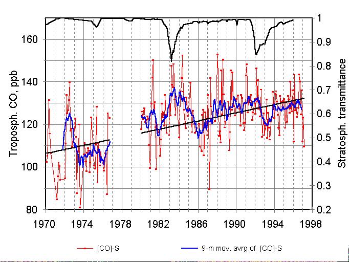
Figure 2. Monthly mean deseasonalized mixing ratios [CO]-S (points)
and 9-months running average (solid curve). Upper curve is the zenith transmittance
of stratospheric aerosol at wavelength 550 nm, calculated from optical
depths for 58.7╨ N, (Hansen et al., 1996).
The unusually high CO values in summer of 1972 have been discussed by
Dvoryashina et al. (1982) and explained by emissions from catastrophic
forest and peat fires in the European part of Russia caused by a strong
drought (Kats, 1974).
Volcanic eruptions of Mt. El-Chichon in April 1982 and Mt. Pinatubo in June 1991 resulted in the injection of large quantities of aerosols into the stratosphere on a global scale. Atmospheric transmittance at the wavelength of 550 nm for the latitudinal belt near 58.7╨ N is plotted at the top of Figure 2 (compiled by Hansen et al.,1996). This data shows that visible (and, obviously, UV) solar radiation was similarly attenuated by the stratospheric aerosol after these eruptions. On the contrary, variations of CO after the eruptions differed not only in magnitude, but even in sign: CO increased after the Mt. El-Chichon eruption and decreased after the Mt. Pinatubo eruption.
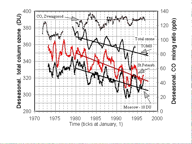
Figure 3. Monthly averaged and deseasonalized (not detrended) total
column ozone in Dobson units (DU) measured from the surface at two sites
in Russia (St. Petersburg, 60o N and Moscow, 56o
N) and from satellites by TOMS instruments. Note that Moscow trace is shifted
down by 10 DU for clarity. Satellite data are zonal averages for the latitudinal
belt 55o - 60o N. CO curve is plotted for comparison.
Solar UV radiation in the spectral range 290 to 330 nm determines the
rate of OH formation in the troposphere. Attenuated UV after the El-Chichon
eruption could be a cause of CO increase in the same period of time. However,
a similar variation of aerosol after the Pinatubo eruption resulted in
quite different behaviour of CO. This leads to a conclusion, that there
should be another mechanism, probably connected with volcanic eruptions,
which influences tropospheric CO.
As was shown by Solomon et al., (1996) (and references therein), volcanic
aerosol particles trigger photochemical heterogeneous reactions, which
destroy ozone molecules in the lower stratosphere. Ozone depletion after
the Pinatubo eruption turned out to be much more pronounced, than after
the El-Chichon eruption because of higher levels of ozone-destructing man-made
chlorine in the stratosphere in 1990s. Both aerosol and ozone attenuate
solar UV; these two mechanisms compete in the net effect on UV changes.
We considered three total ozone data sets for a comparison to the CO data (Figure 3), two of which being measured in Russia. The first one was collected near Moscow (Dolgoprudny) using M83/M124 ozone filter photometers; the second data set was obtained near St. Petersburg (Voyeykovo) by a Dobson spectrophotometer (both archived at the World Ozone and Ultraviolet Radiation Data Centre, WOUDC; WWW site http://www.tor.ec.gc.ca/woudc/woudc.htm). The third data set was measured by TOMS instruments (version 7) on NIMBUS-7 (NASA, 1996a) and METEOR-3 (NASA, 1996b), complemented by recent measurements on the
EARTH PROBE spacecraft between August 1996 and January 1998 (personal
communication, R. McPeters, 1998). These raw data were deseasonalised and
smoothed by the same procedure applied to the CO data (see above). A very
fine correlation can be seen between these three ozone curves (Figure 3),
both for interannual variations and for the long-term trends. In particular,
all three data sets show a drop in ozone with two minima (or a "double
hollow") during 1991 to 1993 after the Pinatubo event. The slopes of the
regression lines in Dobson Units (DU)/ year were TOMS (-1.28 ╠ 0.15); St.Petersburg
(-1.91 ╠ 0.12); Moscow (-1.51 ╠ 0.12). A detailed discussion of the decline
in total ozone after 1980 and interannual variations can be found in Harris
et al. (1997). In our analysis, we have used the TOMS satellite data set,
but the results that would be obtained using other data sets are expected
to be similar.
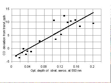
Figure 4. A correlation between deseasonalized and detrended monthly
mean values of CO and aerosol visible optical depth for the period after
El-Chichon eruption (April 1982 - August 1983). Regression line has a slope
of 86 ppb/(unit of optical depth ).
The quasi-linear ozone decline after 1980 could influence CO tropospheric
mixing ratios through an increase in tropospheric UV and OH. What is the
sensitivity of tropospheric CO to changes in the total ozone? It can be
assessed from a correlation between the detrended and the deseasonalized
CO and ozone monthly means. But first it is necessary to correct CO values
to remove the effects of the stratospheric aerosol. A convenient time period
to assess how much CO is effected by changes in aerosol occurred just after
the El-Chichon eruption between April 1982 and August 1983 (Figure 4).
During this time, the total ozone was relatively constant (Figure 3). The
slope of regression line is 86 ╠ 10 ppb per unit of optical depth () (dimensionless).
The r2 correlation coefficient is 0.86.
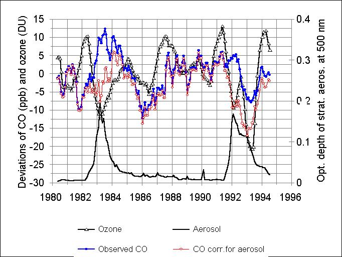
Figure 5. Deseasonalized, detrended and smoothed monthly mean values
of tropospheric CO mixing ratio (full circles) and TOMS total ozone (triangles).
Thick line is the stratospheric aerosol optical depth. Open circles show
CO corrected on aerosol influence.
Figure 5 illustrates the time series of measured deviations of CO (points)
and TOMS ozone (triangles) from their trends. The bottom curve is the mean
zonal optical depth () of the stratospheric aerosol at the wavelength 550
nm for the latitude 58.7° N (Hansen et al.,
1996). CO, corrected for aerosol (open circles), is derived by subtracting
the aerosol contribution (86 ) from the measured CO (points). This contribution
was apparently significant just for the periods after volcanic eruptions
when the optical depth was considerable. Aerosol correction markedly improves
the similarity in shapes between CO and total ozone curves. In particular,
a "double hollow" appears in the CO trace between 1991 and 1993.
A correlation between deviations of the aerosol-corrected CO and ozone
from trends is demonstrated by Figure 6. Here the crosses correspond to
the period between April 1981 and December 1983, and the squares for to
the period between January 1984 and June 1994. The thin regression line
relate to the whole period under consideration between 1981 and 1994 (slope
0.38 ╠ 0.05, intercept -3.188, r2 = 0.25). The thick regression
line is for the period between 1984 and 1994 (squares) (slope 0.53 ╠ 0.058,
intercept -3.992, r2 = 0.41). A worse correlation between ozone
and CO during the first part of the whole period probably can be explained
by the presence of other sources for CO variations and/or imperfect correction
for the stratospheric aerosol. Therefore, the value of 0.53 ppb/DU will
be used in further analysis for the sensitivity of the tropospheric CO
to the changes of total ozone.

Figure 6. A correlation between deseasonalized and detrended monthly
mean values of CO and total column ozone for the period between April,
1981 and December, 1983 (crosses) and between January, 1984 and June, 1994
(squares). Regression line for the entire period 1981-1994 (crosses and
squares) has a slope of 0.38 ppb/DU, the line for the 1984-1994 (just squares)
has a slope of 0.53 ppb/DU.
3.3 How much was the CO trend effected by volcanic eruptions and total ozone trend?
As discussed, both total ozone and aerosol affect tropospheric CO. We
assessed the responses of the CO mixing ratio to unit changes in the stratospheric
aerosol and total ozone. Now we can reduce the measured CO to some constant
levels of these two parameters: namely to zero aerosol and to mean total
column amount of ozone before 1980. Unfortunately, there were no TOMS data
before 1979. Available ground based measurements revealed no trend between
1973 and 1980 (Figure 3). Therefore, we have assumed 370 DU to represent
"undisturbed" zonal ozone annual level at 55°
N.
Grey circles in Figure. 7 relate to measured, deseasonalized and smoothed
(but not detrended) CO mixing ratios. The slope of the regression line
is 0.94 ╠ 0.06 ppb/year (r2 = 0.48). The triangles correspond
to the measured CO subtracted by a "contribution from ozone": ([O3
]- 370 DU) ╢ 0.53 ppb/DU. This curve represents
CO variations assuming stable total ozone. We see in this data two peaks
after both great volcanic eruptions; measured CO has had just one peak.
The regression line corresponding to this case has a slope of 1.45 ╠ 0.07
ppb/year and r2 = 0.67.
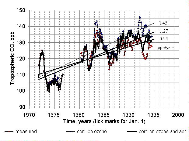
Figure 7. Deseasonalized and smoothed CO mixing ratios and corresponding
regression lines. Red circles and the line with a slope 0.94 ppb/year relate
to measured values. Triangles and the line with a slope of 1.45 ppb/year
relate to CO in assumption of constant total ozone of 370 DU. Thick broken
line and regression with a slope 1.27 ppb/year correspond to CO reduced
to constant ozone and zero aerosol ("no eruptions/ no ozone trend" case).
After the subtraction of a "contribution from aerosol" ( ╢
86 ) we obtain the thick line, which corresponds to CO mixing ratio in
an assumption of an "aerosol-free stratosphere" and stable annual average
of total ozone of 370 DU. In this case, the peaks induced by aerosol disappeared.
The slope of regression line is 1.27 ╠ 0.06 ppb/year (r2 = 0.67).
The residual CO variations, however, are significant. They should be attributed
to other factors influencing tropospheric CO (e.g., production rates) and/or
imperfect correction for ozone and aerosol effects.
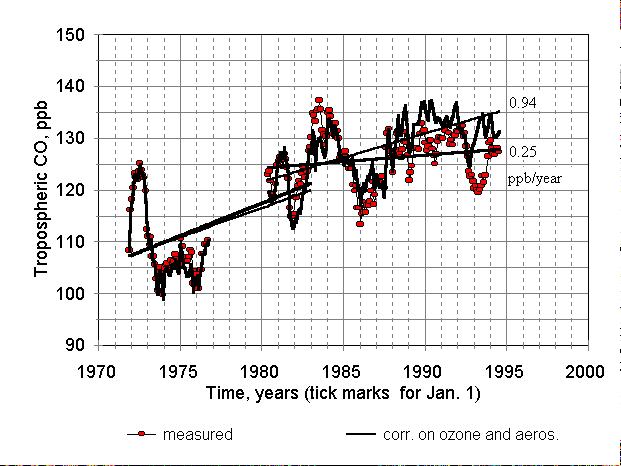
Figure 8. The same as Figure 7 (without triangles), but regression
lines were drawn separately for the first and second parts of the entire
period.
Therefore, the trend in tropospheric CO between 1971 and 1995 was influenced
by stratospheric ozone and aerosol variations. It seems helpful to look
at the stabilisation of CO in 1980s - 1990s, which was probably caused
by the decline in ozone (Figure 8). The slope of regression line, STD and
r2 correlation coefficient for actual CO mixing ratios between
1980 and 1995 are + 0.25 ╠ 0.10 ppb/year, r2=0.04 (i.e. CO is
practically stable). The same parameters calculated for CO mixing ratios,
corrected for variable ozone and aerosol are 0.94 ╠ 0.09 ppb/year, r2=0.40.
For the period between 1971 and 1982 (with a gap in the middle) the slopes
are 1.26 and 1.14 ppb/year with STDs being 0.2 ppb/year (i.e., almost the
same). Thus, the correction for unstable stratospheric composition during
1980-1995 restored the CO trend to a value that is close to 1 ppb/y. However,
residual interannual variations (Figure 8) are still significant. These
variations most likely should be attributed to changes in the NH CO production.
3.4 Comparison to Concurrent Free Tropospheric Colorado Flask Data.
How representative are the total column data obtained in Zvenigorod
and the conclusions made above? As it has been already found by Yurganov
et al.(1998), the correlation between
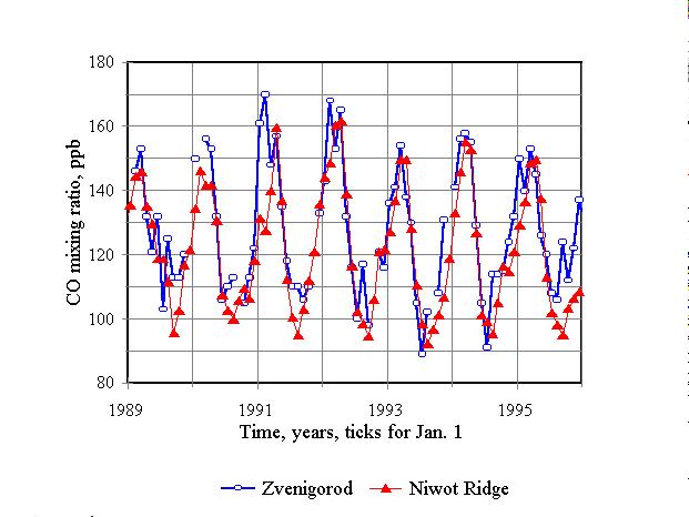
Figure 9. Weighted average CO mixing ratio (mainly tropospheric average),
measured in Zvenigorod, in comparison to free tropospheric mixing ratio
(3475 m asl Niwot Ridge, CO
spectroscopic and surface measurements even at the same place is quite
poor. The most extensive and precise data on worldwide surface-level atmospheric
CO have been collected by the NOAA/CMDL (Novelli et al., 1998). Moreover,
those are mostly measured within the marine boundary layer. Only a few
stations supply data on CO mixing ratio in the free troposphere. Figure
9 illustrates a comparison of spectroscopic CO data, collected at Zvenigorod,
Russia, to CO mixing ratios, measured in Niwot Ridge, Colorado (40°
03' N, 105° 35' W at the height of 3475 m asl)
(Novelli et al., 1998) (the data was obtained from the WWW-site http://www.cmdl.noaa.gov/).
One can see a good correlation between the two data sets (r2=0.74),
especially after January 1991, when the calibration technique, used for
flask analysis, was improved (Novelli et al., 1998). This appears to be
evidence of a good horizontal mixing for the troposphere as a whole in
mid latitudes (much better than for the boundary layer). It is also worth
noting the CO decline after 1991 at both sites, treated in this paper as
a result of the Pinatubo eruption. Mean mixing ratios for the entire seven-year
period of concurrent measurements were 127.8 ppb in Zvenigorod and 121.8
ppb in Niwot Ridge. It is not very surprising, that mixing ratios averaged
over total tropospheric depth turned out to be close to mixing ratio measured
at the height of 3.5 km. However, additional co-located measurements should
be carried out to check this hypothesis.
4. Discussion
Seven years of simultaneous measurements at Zvenigorod, Russia and at
Niwot Ridge, Colorado revealed a very good correspondence of data. This
allows us to extrapolate the conclusions presented above onto the mid-latitude
zonal band. Mean tropospheric CO mixing ratio, measured by solar spectroscopy
in Zvenigorod, increased during last 27 years from 100-110 ppb up to 120-130
ppb.
The increase was not steady. After a peak in 1983 two drops were observed,
thus no significant trend was observed for the period of 1980 - 1995. The
tropospheric CO was found to correlate to total ozone and stratospheric
aerosol. Both these high-altitude species impact on transmission of solar
incoming UV radiation into the troposphere and, therefore, on OH generation
in the troposphere. Sensitivities of CO to changes in ozone and aerosol
were assessed from these correlations: 0.53 ╠ 0.06 ppb CO per 1 DU change
of total ozone and 86 ╠ 10 ppb CO per 1 optical aerosol depth.
The changes in the UV radiation result not just in inter-annual CO variations,
but also in its long-term trend. The latter effect is associated mainly
with a -1.28 DU/year depletion of zonally averaged total ozone near 55°
N after 1980. When the measured CO values were reduced to stable annual
level of 370 DU of total ozone, the CO positive trend restored.
A conclusion was drawn that the observed stabilisation in the CO total
column is associated with an intensification of photochemical sink rather
than with a stabilisation (or even decrease) in the anthropogenic production.
Extensive measurements in the marine boundary layer (Novelli et al.,
1998; Khalil and Rusmussen, 1994) indicated a global decrease of CO mixing
ratio with a rate -2 to -3 ppb/year after 1987. There could be several
reasons for the apparent disagreement with our data. First, the boundary
layer is more strongly influenced by surface CO sources than the total
column amount. Second, some conclusions on CO decline (e.g., Novelli et.
al, 1994) have been made for a relatively short period of time after the
Pinatubo eruption. Total column CO above Zvenigorod underwent a decrease
between 1991 and 1993 also. Third, a possibility of a change in vertical
CO distribution, caused by the global surface temperature warming and more
intensive vertical transport can not be ruled out. Anyway, this difference
seems to be objective and should be taken into account in a treatment of
CO global trends.
What was the rate of OH increase, which was necessary to explain the
change in CO trend? The 0.25 ╠ 0.10 and 0.94 ╠ 0.09 ppb CO per year slopes
(Figure 8) converted into exponential growth correspond to 0.20% and 0.77%
per year. Thus the change of CO trend is 0.57 ╠ 0.19% per year. Assuming
that the reaction with OH is the only tropospheric sink for CO, a similar
per year rate of [OH] increase between 1980 and 1995 would be expected.
The rate was estimated to be 0.6 ╠ 0.3% per year (the precision should
include also uncertainty because of rather poor correlation between CO
and ozone). It is interesting that a very similar estimate of 0.46 % per
year for OH build up with the range of estimate between -0.1 and +1.1%
per year was recently published on the basis of reevaluation of global
methylchloroform measurements between 1978 and 1993 (Krol et al., 1998).
Acknowledgements
The final stage of this work has been supported by a NATO Science Programme
Collaborative Research Grant (CRG 971744). We would also like to thank
Prof. B. Tolton of the University of Toronto for discussion and assistance
in writing this paper.
References
Bekki, S., K.S. Law, and J.A.Pyle, Effect of ozone depletion on atmospheric
CH4 and CO concentrations, Nature, 371, 595-597, 1994.
Conway, T.J., L.P. Steele, and P.C. Novelli, Correlations among atmospheric
CO2, CH4, and CO in the Arctic, March 1989, Atmos.
Environ. 27A, 2881-2894, 1993.
Dianov-Klokov V.I., Spectroscopic studies of atmospheric pollution over
large cities. Izvestia AN SSSR, Fizika atmosfery i okeana, 20, 883-900
(in Russian). 1984.
Dianov-Klokov V.I. and L.N. Yurganov, A spectroscopic study of the global space-time distribution of atmospheric CO, Tellus, 33, 262-273, 1981.
Dianov-Klokov, V.I., and L.N. Yurganov, Spectroscopic measurements of atmospheric carbon monoxide and methane. 2: Seasonal variations and long-term trends, J. Atmos. Chem. 8, 153-164, 1989.
Dianov-Klokov,V.I., L.N. Yurganov, E.I. Grechko, and A.V. Dzhola, Spectroscopic measurements of atmospheric carbon monoxide and methane. 1: Latitudinal distribution, J.Atmos.Chem. 8, 139-151, 1989.
Dlugokencky, E. J., E.G. Dutton, P.C. Novelli, P.P. Tans, K.A. Masarie, K.O. Lantz, and S. Madronich, Changes in CH4 and CO growth rates after the eruption of Mt.Pinatubo and their link with changes in tropical tropospheric UV flux, Geoph. Res. Lett. 23, 2761-2764, 1996.
Dvoryashina E.V., V.I. Dianov-Klokov and L.N. Yurganov, On the variations of total column carbon monoxide during 1970-1982, Izv. Acad. Sci. USSR, Atmos. Oceanic Phys., Engl. Transl. 20, 27-33, 1984.
Fokeeva E.V., E.I. Grechko, and M.S. Pekur, Air pollution in the center of Moscow in the fall: Carbon monoxide, Izv. Acad. Sci. USSR, Atmos. Oceanic Phys., Engl. Transl., 34, 508-515, 1998.
Haan, D., P. Martinerie, and D. Reynaud, Ice core data of atmospheric carbon monoxide over Antarctica and Greenland during the last 200 years, Geophys. Res. Lett., 23, 2235-2238, 1996.
Hansen, J. et al., A Pinatubo climate modelling investigation, in The Mount Pinatubo Eruption: Effects on the Atmosphere and Climate, edited by G. Fiocco, D. Fua, and G. Visconti, pp. 233-272, NATO ASI Series Vol. I 42, Springer-Verlag, Heidelberg, Germany, 1996.
Harris, N.R.P. et al., Trends in stratospheric and free tropospheric ozone, J. Geophys. Res., 102, 1571-1590,1997.
Harris, R.C. et al. Carbon monoxide and methane over Canada: July-August 1990, J. Geophys. Res. 99, 1659-1670, 1994.
Kats, A.L., Neobychnoye leto 1972 goda (Unusual summer of 1972), (In Russian), 75 pp., Gidrometeoizdat, Moscow, 1974.
Khalil M.A.K., and R.A. Rasmussen, Carbon monoxide in the Earth`s atmosphere: indications of a global increase, Nature 332, 242-245, 1988.
Khalil, M.A.K., and R.A.Rasmussen, Global decrease in atmospheric carbon monoxide concentration. Nature, 370, 639-641, 1994.
Khalil, M.A.K., and R.A. Rasmussen, The changing composition of the Earth's atmosphere, in Composition, Chemistry, and Climate of the Atmosphere, edited by H.B. Singh, pp. 50-87, Van Nostrand Reinhold, New York, NY, 1995.
Kroll, M., P.J. van Leeuwen, and J. Lelieveld, Global OH trend inferred from methylchloroform measurements, J. Geophys. Res. 103, 10,697-10,711, 1998.
Logan, J.A., M.J. Prather, S.C. Wofsy, and M.B. McElroy, Tropospheric chemistry:: a global perspective, J. Geophys. Res. 86, 7210-7254, 1981.
Madronich, S., and C. Granier, Impact of recent ozone changes on tropospheric ozone photodissociation, hydroxyl radicals, and methane trends, Geophys. Res. Lett. ,19, 465-467, 1992.
Migeotte M.V., The fundamental band of carbon monoxide at 4.7 ╣m in the solar spectrum, Phys. Rev. 75, 1108-1109, 1949.
Mueller J.-F., and G.Brasseur, IMAGES: a three-dimensional chemical transport model of the global troposphere, J. Geophys. Res. 100, 16,445-16,490, 1995.
NASA, Goddard Space Flight Center, TOMS Version 7, Gridded O3 Data: 1978-1993, R. McPeters and E.Beach, Eds., May 22, 1996, CD-ROM edition, 1996a.
NASA, Goddard Space Flight Center, Meteor 3/TOMS Version 7, O3 and Reflectivity Data: 1991-1994, R. McPeters and E.Beach, Eds,, CD-ROM edition, 1996b.
Novelli, P.C., L.P. Steele, and P.P. Tans, Mixing ratios of carbon monoxide in the troposphere, J. Geophys. Res. 97, 20731-20750, 1992.
Novelli, P.C., K.A. Masarie, and P.M. Lang, Distributions and recent changes in atmospheric carbon monoxide, J. Geophys. Res., 103,19,015-19,033, 1998.
Pougatchev N.S., and C.P. Rinsland, Spectroscopic study of the seasonal variation of carbon monoxide vertical distribution above Kitt Peak, J. Geophys. Res. 100, 1,409-1,416, 1995.
Rodgers, C.D.,. Characterization and error analysis of profiles retrieved from remote sounding measurements, J. Geophys.. Res., 95, 5587-5595, 1990.
Rothman L.S. et al., The HITRAN database: 1986 edition, Appl.Opt. 26, 4058-4097, 1987.
Rothman L.S. et al., The HITRAN molecular database: editions of 1991 and 1992, J.Quant.Spectrosc. Radiat. Transfer 48, 469-508, 1992.
Seiler W., The cycle of atmospheric CO, Tellus, 26, 116-135, 1974.
Solomon, S., R.W. Portmann, R.R. Garcia, L.W. Thomason, L.R.Poole, and M.P. McCormick, The role of aerosol variations in anthropogenic ozone depletion in northern mid-latitudes, J. Geophys. Res.,101, 6713-6727, 1996.
Yonemura, S., and N. Iwagami, Infrared absorption measurement of carbon monoxide column abundance over Tokyo, Atmos. Environ. 27A, 30, 3697-3703, 1996.
Yurganov L.N., E.I. Grechko, and A.V. Dzhola, Carbon monoxide and total ozone in Arctic and Antarctic regions: seasonal variations, long-term trends and relationships, The Sci. of the Total Environ. 160/161, 831-840, 1995.
Yurganov L.N., E.I. Grechko, and A.V. Dzhola, Variations of carbon monoxide density in the total atmospheric column over Russia between 1970 and 1995: upward trend and disturbances, attributed to the influence of volcanic aerosols and forest fires. Geophys. Res. Lett. , 24, 1231-1234, 1997.
Yurganov L.N., D.A. Jaffe, E. Pullman, and P.C. Novelli, Total column and surface densities of atmospheric carbon monoxide in Alaska, 1995, J. Geophys. Res., 103 , p. 19,337-19,346, 1998.
Zander, R., P. Demoulin, D.H. Ehhalt, U. Schmidt, and C.P. Rinsland,
Secular increase of total vertical column abundance of carbon monoxide
above central Europe since 1950, J. Geophys. Res. 94 , 11021-11028,
1989.