Appendix A: Two Versions of the Spectroscopic Technique
There may be a difference in CO determination using two different techniques from the same spectrum. The current computer algorithm is a successor of manual algorithms, which were developed by Pugachev et al. [1978] and Dianov-Klokov et al. [1989]. Those techniques derived CO and H2O contents from the area of a triangle, drawn manually as close as possible to the real shape of a spectral line. A relation between the triangle's area (W) and total column gas content (U) was represented as:
U = W2 (m * A) -1 (P/1013) -1.5, (A1),
where m is the air mass (number of air molecules along the slant path,
related to that in the vertical column), and A is a calibration coefficient,
derived from spectra, simulated using line-by-line layer-by-layer computation
and the HITRAN 1986 spectroscopic database.
The dependence of U on W2 in (A1) is not exact; a possible deviation
from this may be as high as 2-3 %. The second source of disagreement between
two techniques is using different line parameters.
Examples of raw data for May 1, 1995, processed by two techniques, are
presented in Fig. A1.
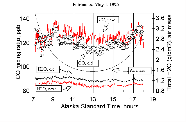
Fig. A1. Carbon monoxide (left scale) and water vapor (right scale ) individual total column measurements in Fairbanks, May 1, 1995, processed by two techniques. "Old" means the technique used previously [Dianov-Klokov et al, 1989]. "New" means the technique described and used in this paper. Air mass = 1/cos (z) is also shown by a solid curve (right scale).
"New" technique is the present code, described in the section Experimental. The "old" one is a computer simulation of the old manual technique [Dianov-Klokov et al., 1989]. As a rule, absolute values of CO mixing ratio for both techniques are close to one another for air masses between 2 and 3.6, but new data are 7% higher than old ones for air masses between 1.6 and 2. The difference for H2O determinations (bottom two curves) using a weaker line does not depend on air mass and, most probably, is caused by different parameters of spectral lines. A correlation between the two techniques on the basis of more than 6,000 spectra is illustrated by Table A1.
TABLE A1. Ratios of CO abundances,
determined by two techniques, and their standard deviations.
| Month, 1995 | Number of spectra | Mean air mass | New/old | STD |
| March | 399 | 2.73 | 0.960 | 0.009 |
| April | 1338 | 2.25 | 1.013 | 0.023 |
| May | 1980 | 1.85 | 1.066 | 0.020 |
| June | 1035 | 1.63 | 1.077 | 0.023 |
| July | 696 | 1.65 | 1.045 | 0.028 |
| August | 187 | 1.70 | 1.061 | 0.006 |
Appendix B. Some Systematic Errors.
Uncertainties due to Unknown CO Profiles.
Real atmospheric CO profiles are quite variable. If we assume that CO mixing ratio is constant for all the heights (as we do here and did in our previous papers), we introduce an error in our results. As was noted by Pugachev [1988], spectroscopically measured total column amount is in fact a weighted mean amount (or weighted mean mixing ratio <R>) rather than an actual mean. If a constant with height a-priori profile is assumed, then:
 (B1)
(B1)
Here R(P) is the molar mixing ratio, P is air pressure, P0
and P1 are bottom and top air pressures, respectively. F(P)=
d(<R>)/dR , is a weighting function (WF). When F(P) = 1,
this is the actual mean.
WFs for the R(3) line, resolution 0.2 cm-1 (Fig.B1) have been
calculated using an algorithm described by Pugachev
[1988]. Winter and summer WFs were calculated for air masses equal
to 5 and 1.3, mixing ratios for the entire atmosphere 180 ppb and 100 ppb,
respectively, and winter and summer typical air temperatures and humidities.
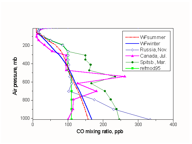
Fig. B1. Weighting
functions (WF) of IR spectrometer, calculated for typical winter and summer
conditions and examples of CO vertical distributions, modeled and observed
(see text).
Reference profiles, plotted in Fig. B1, are close to those measured
between the boundary layer and 6-7 km of altitude, and extrapolated to
higher levels. The Russian profile was acquired at a location about 100
km southeast of Moscow (54.9 N, 35.5 E) in November, 1995 [Tans
et al., 1996]. It seems to be typical for a continental region with
moderate pollution. The Canadian profile was measured on July 21, 1990
(56N, 105W, Mauzerall et al. [1996]). Polluted
layers at 700 and 500 mb most likely are of forest fire origin. The Spitsbergen
profile for March 21, 1989, reported by Conway et
al. [1993], illustrates a case of the Arctic atmosphere, polluted by
a long-range air transport. The profile "refmod95" is a standard
model CO profile, used by SFIT procedure [Rinsland
et al., 1982]. It is close to a well-mixed troposphere.
These profiles have been convolved with the WF (eqv. B1, Table B1, col.
4). Columns 2 and 3 contain actual averages for total atmosphere and troposphere,
respectively.
TABLE B1. Average mixing ratios of CO, which would be measured using R(3) spectral line, constant assumed profile and different actual vertical CO profiles.
| Row | Profile | Actual average,
1013-0 mb |
Actual trop. average.
(0-10 km, 1013-265 mb ) |
Weighted aver., (1013-0mb) (eq. B1) | C.4/C.2 | C.4/C.3 |
| 1 | 2 | 3 | 4 | 5 | 6 | |
| 1 | Russia, Novem. | 123.6 | 167.3 | 153.0 | 1.24 | 0.91 |
| 2 | Canada, July | 102.1 | 129.4 | 119.4 (121.9) | 1.17(1.19) | 0.92(0.94) |
| 3 | Spitsberg., Mar. | 159.0 | 196.8 | 192.2 | 1.21 | 0.98 |
| 4 | refmod95 | 92.5 | 106.8 | 104.1 | 1.12 | 0.97 |
Note. Rows 1, 3, 4 have been calculated using the winter WF; row 2,
using summer WF and winter WF (in parenthesis): the difference is less
than 2%.
According to these calculations, CO mixing ratio, measured spectroscopically
with the constant assumed a-priori profile, should always be higher than
the actual total column average. Second, for the Arctic profile, as well
as for the well mixed troposphere, weighted averages are very close to
actual averages for the troposphere (the error is less than 2-3%). In the
cases when polluted layers are present either in the boundary layer or
aloft, spectroscopy should underestimate real tropospheric burden, but
not more than 9%.
Uncertainties due to Line Constants
As was mentioned previously, an absolute accuracy of total column measurements strongly depends on the intensities of spectral lines. The lines of influence for the interval 2157.0 - 2159.0 cm-1 are (i) CO R(3), (ii) a few N2O lines, (iii) H2O line near 2158.105 cm-1, (iv) solar CO lines. Variations in the CO line intensity and halfwidth seem to be the most important. HITRAN databases were improved from one version to another. CO parameters for different versions are shown in Table B2.
TABLE B2. Parameters of the R(3) line of CO fundamental band
from different versions of the compilation HITRAN.
| Version of HITRAN | vo, Line center, cm-1 | S, Line intensity,
cm-1 mol-1 cm-2 |
a, Lorentz Half-width, cm-1 atm-1 | S*a | S*a, relat. to HITRAN 1992 |
| 1986 | 2158.3000 | 3.29E-19 | 0.077 | 2.5333E-20 | 1.094 |
| 1992 | 2158.2997 | 3.47E-19 | 0.0667 | 2.31449E-20 | 1.000 |
| 1996 | 2158.2997 | 3.339E-19 | 0.0667 | 2.22711E-20 | 0.962 |
CO abundance is roughly proportional to 1/S*a, where S is the line intensity and a is the Lorents half-width . Using the HITRAN 1996 version, which is the most recent one, would result in 4 % higher CO abundance than the 1992 version in this paper. On the other hand, the version of 1986 (Rothman et al, 1987), which was used in our old technique, would give values 9% lower than the 1992 version. This is in general agreement with the comparison between the techniques, which was performed previously (Fig. A1 and Table A1).
The total contribution of the N2O lines to the EQW is about 15%. If the uncertainty of N2O line parameters is ±10%, then it can contribute an additional 1.5-2% uncertainty into CO determination. The uncertainty in the solar CO contribution is even less. A special calculation revealed that neglecting CO solar lines changes the measured CO abundance less than 2%. A contribution of the H2O line becomes significant (up to 15-20%) only for maximum humidities (a few days per year in mid or high latitudes). Even for these days the uncertainty in the H2O parameters can not change the CO value more than 2%.
Therefore, we can expect that the uncertainty in line parameters' data could result in a possible bias in a CO determination of ±(5-10)% at most.