2.2 Comparisons between aircraft-borne, balloon-borne, and ground-based sensors
2.2.1 Stratospheric measurements
NOAA-AL Lyman-a and NOAA-CMDL frostpoint hygrometer
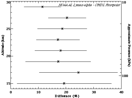
There have been eight coincident flights between the NOAA Aeronomy Laboratory (AL) Lyman-a instrument and the NOAA Climate Monitoring and Diagnostics Laboratory (CMDL) frostpoint balloon instrument. In the early 1980's, these used both a Lyman-a balloon instrument and an aircraft instrument. Coincident comparison flights occurred in Texas, Wyoming and California. The percent difference as a function of altitude between 15 and 30 km is shown in Figure 2.1. Differences are on the order of 20%, with the Lyman-a instrument measuring larger values.
Figure 2.1. Percent difference between the NOAA-AL Lyman-a and NOAA-CMDL frostpoint balloon instruments. 8 comparison flights were included in this calculation. Data from all flights were put into 2-km bins, the mean is shown by the symbol, and the standard deviation (1s) denoted by the horizontal lines. Percentage differences were calculated by taking (AL-CMDL)/average.
Harvard Lyman-a and NOAA-CMDL frostpoint hygrometer
There are only a few comparisons between the Harvard Lyman-a ER-2 and NOAA-CMDL frostpoint instruments. The only direct comparison consists of three flights in May 1993 at Crows Landing, California, as part of the SPADE aircraft mission. The same 3 days are also included in the NOAA-AL:NOAA-CMDL comparison. Percent differences between the Harvard and NOAA-CMDL instruments are shown in Figure 2.2. There is a wide range of percentage differences as a function of altitude, the average being 27%, with Harvard values larger.
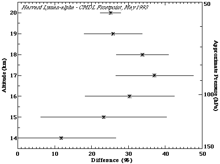
Figure 2.2. Percent difference between the Harvard Lyman-a and NOAA-CMDL frostpoint balloon instruments. 3 comparison flights were included in this calculation. Data from all flights were put into 1-km bins, the mean is shown by the symbol, and the standard deviation (1s) denoted by the horizontal lines. Percentage differences were calculated by taking (Harvard-CMDL)/average.
The only other near coincidences between the Harvard and NOAA-CMDL instruments were during the Central Equatorial Pacific Experiment (CEPEX) campaign in the equatorial Pacific during March 1993. In this case, there were no geographic coincidences, but the two instruments were both measuring in the same general area. For this comparison, all the NOAA-CMDL measurements were averaged into one profile, as were all the Harvard measurements. The offset between the two instruments is ~1.4 ppmv, with the Harvard measurements greater. This amounts to approximately a 30% difference at ER-2 cruise altitudes (near 20 km) and over 40% differences at lower altitudes near the hygropause. Gradients in satellite measurements taken during the same month across the Central Pacific near 20 km are less than 0.1 ppmv across the width of the basin. It is therefore unlikely that the differences noted between the two in situ measurements at ER-2 cruise altitudes are a result of geographic biases, but instead indicative of an actual measurement difference.
Jülich Lyman-a (FISH) and LMD frostpoint
Balloon-borne profiles of the Jülich Lyman-a fluorescence hygrometer FISH and the LMD frostpoint hygrometer can be compared using 2¥CH4+H2O even when data are not sampled in spatial and temporal coincidence. For a number of flights of both hygrometers, CH4 was measured by the same whole air sampler instrument with gas chromatographic analysis traceable to a single standard [Schmidt et al., 1987]. Given a precision of better than 3% for the CH4 measurement and assuming variations of 2¥CH4+H2O in the middle stratosphere (420-700 K) at mid- to high latitudes covering the period of a few years are of the same magnitude, discrepancies of more than 5% between the H2O measurement techniques should be detectable.
A series of balloon flights of the LMD frostpoint and the whole air samplers during the European Arctic Stratospheric Ozone Experiment (EASOE) in winter 1991/92 at 68°N has been used to determine 2¥CH4+H2O [Engel et al., 1996]. This quantity was found to be 6.91±0.41 ppmv at potential temperatures from 430 K to 750 K. There were no significant differences between data obtained inside or outside of the polar vortex. From a mid-latitude balloon profile on 20 September 1993 using FISH and the whole air sampler, 2¥CH4+H2O was determined to be 7.17±0.62 ppmv for potential temperatures ranging from 420 K to 900 K [Zöger et al., 1999b]. Two more flights of this payload at 68°N yielded a value of 7.02±0.11 ppmv (11 February 1997, 400-600 K) and 7.05±0.12 ppmv (6 February 1999, 420-580 K). LMD frostpoint measurements are slightly smaller than FISH data by 0.1-0.2 ppmv.
In May 1999, both hygrometers were launched on balloons from Southern France within 60 hours of one another. Despite a few filamentary structures which differ in both profiles due to atmospheric variability, Figure 2.3 shows that both measurements agree to within 0.2 ppmv at 90-50 hPa with a maximum deviation of 8%.
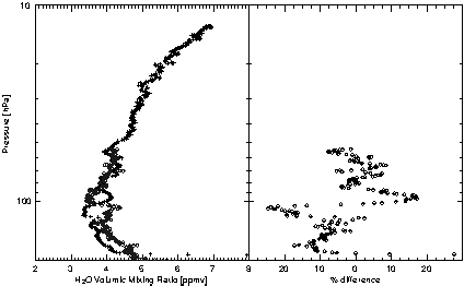
Figure 2.3 Intercomparison of H2O balloon profile measurements of the LMD frostpoint hygrometer (crosses, 5th May 1999) and of the Jülich Lyman-a hygrometer (open diamonds, 3 May 1999) at 44°N.
NOAA-AL and Harvard Lyman-a on the ER-2
During the NASA SPADE mission (April-May 1993), both Harvard and NOAA-AL Lyman-a instruments flew on the ER-2 high altitude aircraft. The average difference over the nine flights used in this comparison is ~15%, with the Harvard measurements larger. The offset in mixing ratio is ~0.7 ppmv. The vertical distribution of the percent differences is shown in Figure 2.4. Percent differences are fairly constant with altitude above 15 km. Comparisons of measurements below 15 km taken during aircraft ascent and descent show more vertical structure and greater variability in the differences. As discussed later in the laboratory intercomparison (2.2.2), the reasons for the disagreement are not understood, nor reproducible under controlled laboratory conditions.
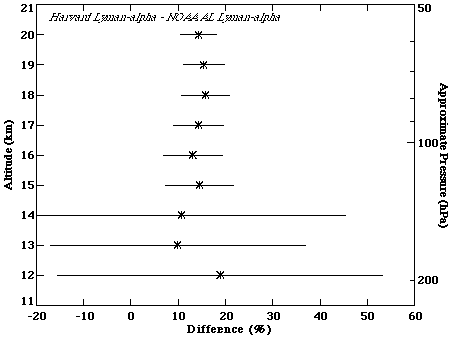
Figure 2.4 Percent difference between the Harvard and NOAA-AL Lyman-a instruments flying on the ER-2 during SPADE. 9 comparison flights were included in this calculation. Data from all flights were put into 1-km bins, the mean is shown by the symbol, and the standard deviation (1s) denoted by the horizontal lines. Percentage difference is calculated by taking (Harvard-AL)/average.
Lyman-a and JPL TDL
During the NASA POLARIS mission (April-September 1997), the Harvard Lyman-a instrument was compared with the TDL hygrometer from JPL [May, 1998; Hintsa, 1999]. Average agreement for the entire June-July deployment was 1% from 0-200 ppmv H2O with an offset of less than 0.2 ppmv; most measurements agreed to within 5%. Nonetheless, there were significant pressure-dependent differences at pressures between 100 and 300 hPa as shown in Figure 2.5, where the Harvard instrument measured less than the JPL instrument. These are thought to arise from uncertainties in the modulation amplitude placed on the diode laser for second harmonic detection. Using a fixed modulation amplitude produces a pressure-dependent uncertainty because of undermodulation at higher pressures. Some variation is seen between deployments during POLARIS, especially at pressures greater than 100 hPa. At cruise altitudes (19-21 km), where water is low and the JPL TDL calibration was most reliable, the agreement is within 1% with an offset of < 0.1 ppmv.
During the NASA/NOAA WBS7F Aerosol Mission (WAM) mission (April 1998), the NOAA-AL Lyman-a and JPL TDL hygrometers had two coincident flights on the WB57F high altitude aircraft. Considering data just above 15 km, the average difference is 16%, with the JPL TDL measurements larger. If the entire altitude range is considered, the average difference is ~10%. This reflects the vertical structure in the percent differences, plotted in Figure 2.6. The shape is similar to that in the percent differences between the Harvard Lyman-a and JPL TDL instruments shown in Figure 2.5, except offset by 10-15%. Reasons for the pressure-dependent differences are discussed above. In spite of these differences, the JPL TDL instrument can be used as a transfer agent between the Harvard and NOAA-AL Lyman-a instruments. This comparison would also indicate that the differences between the Harvard and NOAA-AL Lyman-a instruments would be ~15%, with the Harvard instrument larger.
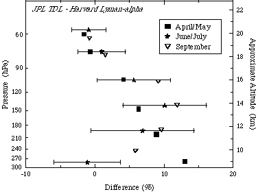
Figure 2.5 Percent difference between the JPL TDL and Harvard Lyman-a instruments flying on the ER-2 during POLARIS in 1997. Data from 0 to 200 ppmv H2O from all flights are included in this calculation, with the mean shown for each deployment: April/May (squares), June/July (stars), and September (triangles). The standard deviation (1s) is denoted by the horizontal lines. Percentage difference is calculated by taking (JPL-Harvard)/average.
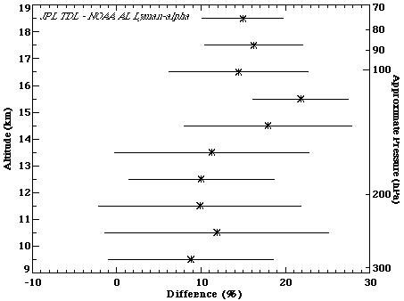
Figure 2.6 Percent difference between the JPL TDL and NOAA-AL Lyman-a hygrometers. Two comparison flights were included in this calculation. Data from both flights were put into 1-km bins, the mean is shown by the symbol, and the standard deviation (1s) denoted by the horizontal lines. Percentage difference is calculated by taking (JPL-AL)/average. Data was binned in altitude space, but plotted in pressure space for easier comparison with Figure 2.5.
2.2.2 Laboratory intercomparison of the NOAA-CMDL, NOAA-AL, and Harvard in situ instruments
Because atmospheric comparisons between the NOAA-CMDL frostpoint hygrometer and the NOAA-AL and Harvard Lyman-a instruments (discussed in section 2.2.1) showed systematic differences with the frostpoint smaller, several laboratory intercomparisons were conducted to study this problem under controlled conditions. The goal of the laboratory intercomparisons was to investigate potential systematic differences between instruments in a controlled environment that attempted to duplicate atmospheric conditions. These laboratory measurements covered a wide range of parameters, with the hope of identifying the source of the disagreement. The set-up relied on simultaneous measurements of the same air source, rather than an independent mixing ratio standard, which may itself not be reliable. This allowed a limited systematic investigation of the behaviour of each instrument under varying conditions. These experiments tested whether the disagreement between the instruments depends on water vapour mixing ratio, pressure, and temperature, on CO2 and methane concentrations, on flow rate, and on several instrument parameters.
The three instruments are described in detail in Chapter 1. All three instruments operate under different temperature conditions during flight and use different calibration procedures. The NOAA-AL Lyman-a hygrometer is a temperature-controlled instrument, including heated intake lines. The instrument performs calibration cycles at regular intervals during flight. A modified version of the NOAA-CMDL frostpoint hygrometer balloon instrument was built to operate in a laboratory configuration. It was calibrated and operated at ambient temperatures as described in Chapter 1, however, for practical reasons, a different cryogen (liquid nitrogen) was used. The Harvard Lyman-a hygrometer operates at slightly above ambient temperature in flight with calibrations performed in the laboratory before and after atmospheric measurements. Attempts were made in the laboratory, but with varying degrees of success, to bring air into the instruments in a way similar to flight operation. Accordingly, this provides a potential source of uncertainty when comparing flight and laboratory operation for all three instruments.
While the two Lyman-a hygrometers measure mixing ratio directly, the frostpoint hygrometer measures the frostpoint temperature, which has to be converted to mixing ratio using a form of the Clausius-Clapeyron equation as well as an independent pressure measurement. The Goff-Gratch formula [List, 1949], which agrees to within 2% with the most recent direct measurements by Marti and Mauersberger [1993], was used to convert frostpoint temperature to water vapour partial pressure. The pressure measurements were accurate to within 1%, and thus the error introduced by the conversion of frostpoint temperature to mixing ratio is less than 3%.
On several occasions, test runs were influenced by contamination from the outgassing of lines in the flow system. However, this was always due to extremely low flow rates or insufficient settling times after closing the flow system or after sudden changes in mixing ratio. These runs did not give any indication that contamination could be a source of the disagreement in atmospheric measurements. No experimental run reproduced the disagreement between any of the three instruments and all measurements agreed to well within the instrumental uncertainties. A summary of these runs is shown in Figure 2.7.
The laboratory comparisons did not reveal the cause of the systematic difference between the three instruments in atmospheric comparisons. Under the controlled conditions of the laboratory, all instruments agreed to within the instrumental uncertainty. The average difference between the NOAA-CMDL frostpoint hygrometer and the NOAA-AL Lyman-a hygrometer was 3.3±5% (1s), while the difference between the frostpoint hygrometer and the Harvard Lyman-a was 4.4±5.0 % (frostpoint smaller). This is based on mixing ratios greater than 5 ppmv. At lower mixing ratios, the laboratory configuration and difficulty in controlling the dry air source led to much greater scatter in the differences as can be seen in Fig 2.7. The 15% difference between the NOAA-CMDL frostpoint and the NOAA-AL Lyman-a hygrometer, as well as the 15% difference between the NOAA-AL and the Harvard Lyman-a hygrometer in atmospheric measurements could not be reproduced in laboratory measurements. Tests between the NOAA-CMDL frostpoint and the NOAA-AL Lyman-a hygrometer were run to determine whether differences depend on temperature, pressure, mixing ratio, or other trace gases. No such dependence was found. Tests were run to determine whether the agreement found in the laboratory could have been caused by the differences in the set-up compared to atmospheric measurements. None of the instruments appeared to have inherent biases and seemed to be capable of measuring low water vapour concentrations accurately under controlled laboratory conditions. The differences in atmospheric measurements remain unexplained, but are most likely connected to the installation on the respective platform. Outgassing is of concern, but no indication of such a problem connected to the installation on the respective platforms was found. This disagreement still needs to be resolved to allow accurate and reliable measurements of water vapour in the stratosphere.
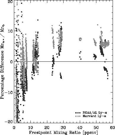
Figure 2.7 The percentage difference in water vapour mixing ratio measured by the NOAA-AL Lyman-a hygrometer and the Harvard Lyman-a hygrometer as a function of the water vapour mixing ratio measured by the NOAA-CMDL frostpoint hygrometer.
2.2.3 Balloon infrared instrument comparisons
MIPAS intercomparisons
Balloon-borne profile measurements of water vapour using the MIPAS payload and the LMD frostpoint hygrometer have been made within 48 hours of each other (11 February 1995 and 13 February 1995) at 68°N [Stowasser et al., 1999]. Figure 2.8 shows the retrieved profile measurements of both instruments. At nearly all stratospheric altitudes, the difference is less than 0.2 ppmv, except at 80 hPa where the LMD frostpoint instrument encountered a laminae of dry air that was probably not present during the MIPAS balloon flight two days before.
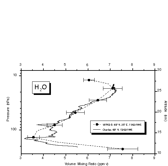
Figure 2.8 H2O profiles retrieved from two MIPAS-B flights inside the Arctic vortex in 1995 and 1997. The 1995 profile is compared to an in situ measurement obtained two days later at the same location [Ovarlez and Ovarlez, 1996]. Errors bars denote the 1s confidence limit and include random noise, mutual influence of fitted parameters, temperature and pointing uncertainties, and onion-peeling error propagation, but not errors in spectroscopic data. Figure adopted from Stowasser et al. [1999].
In 1997, several balloon-borne measurements using different techniques were made for validation of the ADEOS-ILAS satellite programme. Even though further improvements of the retrieval of ILAS water vapour are under development, the currently available data can be used as an independent reference measurement (see section 2.3.5). A MIPAS balloon instrument measurement was taken on 24 March 1997 at 68°N, approximately 560 km from an ILAS overpass. Between 16-20 km, both water vapour profiles agree within 0.2 ppmv. At higher altitudes, ILAS data are larger than MIPAS. For example, the difference at 25 km is approximately 0.5 ppmv. Similar qualitative and quantitative results were observed on 11 February 1997 using the Jülich Lyman-a hygrometer (FISH) measuring at a distance approximately 140 km from an ILAS overpass. Using ILAS as a transfer standard, indirect evidence is provided that MIPAS and FISH measurements do not differ by more than 0.3 ppmv in the lower and middle stratosphere.
From the MIPAS measurements, a mean mixing ratio of 2¥CH4+H2O was determined to be 7.25± 0.2 ppmv (11 February 1995) and 7.28± 0.1 ppmv (24 March 1997) [Stowasser et al., 1999]. These values are within 0.3 ppmv of those determined for FISH and the LMD frostpoint (see section 2.2.1). Since no obvious discrepancies for the CH4 techniques greater than 0.1 ppmv have been observed [Stowasser et al., 1999], differences in the sum 2¥CH4+H2O largely reveal differences in the water vapour measurements. Therefore, it appears that the LMD frostpoint, FISH, and MIPAS, all based on independent techniques, give results within 0.2-0.3 ppmv.
MkIV and aircraft comparisons
The JPL MkIV interferometer flew from Fairbanks, Alaska in May 1997 during the Photochemistry of Ozone Loss in the Arctic Region in Summer (POLARIS) campaign. MkIV is a balloon-borne FTIR spectrometer operated in solar occultation mode. The instrument is described more fully in Chapter 1. Several ER-2 flights took place within a few days of the MkIV balloon flight. Two instruments on the ER-2 measured water vapour during POLARIS, the JPL TDL hygrometer and the Harvard Lyman-a hygrometer. Only those data acquired within approximately 500 km of the balloon observations, which were well outside the polar vortex in a region of uniform potential vorticity were considered for the comparison presented in Figure 2.9. Data is compared as a function of CH4 (from both the MkIV and ALIAS instruments) to minimise variations due to differences in airmass origin. Additionally, the MkIV CH4 was scaled by 0.975 to eliminate a bias reported by Toon et al. [1999]. Data points having a potential temperature less than 375 K were excluded from this comparison, to avoid any tropospheric airmasses, where spatial gradients are known to be greater. Although these results show significant variability from flight to flight (which may well be real), in general the aircraft in situ H2O measurements are 0 to 20% larger than those measured remotely by MkIV, with the bias largest near the tropopause.
FIRS-2 and aircraft comparisons
The FIRS-2 spectrometer flew from Fairbanks, Alaska, on 30 April 1997 as part of the Alaska Balloon Campaign in support of the ADEOS satellite. The balloon campaign overlapped in time with the POLARIS campaign, and the NASA ER-2 was flying near Fairbanks when FIRS-2 was launched. FIRS-2 measurements were obtained 6°N of the aircraft flight track, but within the longitude range covered by the ER-2, providing an opportunity for intercomparison. The balloon profiles were obtained well outside the vortex, and back trajectory calculations show that the flow was out of the south at all altitudes sampled by the ER-2, so that mixing ratio gradients were small between the ER-2 flight track and FIRS-2 measurement locations. In addition, ILAS measurements made at the same latitude as the ER-2 measurements are consistent with FIRS-2 measurements (section 2.3.5.), again suggesting that local gradients were small.
The ER-2 flight on 30 April consisted of the climb out of Fairbanks, 5.5 hours of level flight between the 490 K and 510 K potential temperature surfaces, and the descent back into Fairbanks. Roughly half the flight took place before sunrise. The aircraft payload included both the JPL TDL and Harvard Lyman-a water vapour instruments, as well as the ALIAS instrument from JPL. ALIAS provided measurements of N2O, among other species.
Because a remote sensing balloon instrument provides measurements at a limited spatial resolution, it will underestimate the amplitude of small-scale variability in a heterogeneous airmass at a given altitude, unlike the aircraft in situ measurements. It is possible to compensate for some of the variability mismatch by comparing correlations with a long-lived tracer like N2O, but only if the relationship is independent of airmass origin. This is not the case for the correlation between H2O and N2O. In the tropics, the annual cycle causes the correlation to depend on altitude and season at all altitudes accessible to the ER-2. Outside the tropics, the difference between vortex and middle latitude correlations relating CH4 and N2O [Michelsen et al., 1998] causes a complementary dependence in the relationship between H2O and N2O.
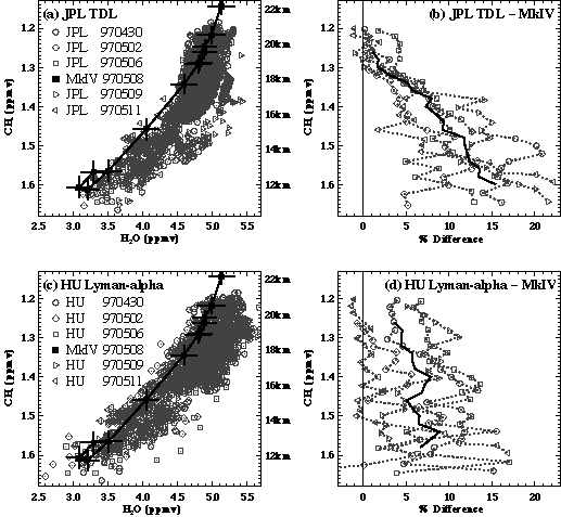
Figure 2.9 Comparison of H2O profiles measured by MkIV with those measured by two in situ instruments on board the NASA ER2 above Fairbanks, Alaska in May 1997. The profiles are plotted as a function of CH4. Approximate altitude is also given. The top panels are comparisons with the JPL TDL hygrometer, the bottom panels with the Harvard Lyman-a hygrometer. The left-hand panels show the measurement, black squares in the left hand panels are from the JPL MkIV interferometer, the other points are the in situ aircraft measurements. The right panels show percent average biases between the MkIV measurements and 5 aircraft flights, the grand average bias is given by the black solid line.
However, similar airmasses have been identified by binning the data by both potential temperature and N2O mixing ratio. The ascent and descent data are binned separately by potential temperature and compared with FIRS-2 profiles for H2O in the top panels of Figure 2.10. The nighttime and daytime cruise data are binned separately by N2O and compared in the middle panels of Figure 2.10 with the H2O-N2O relationship observed by FIRS-2. As shown in the bottom panel of Figure 2.10, cruise data obtained at N2O mixing ratios between 200 and 215 ppbv are most similar (on the basis of potential temperature and N2O mixing ratio) to the airmasses observed by FIRS-2.
The H2O mixing ratio retrieved by both in situ instruments is systematically smaller after sunrise, with the JPL TDL measurements showing a larger change. Above 450 K the average water vapour mixing ratio measured by FIRS-2 is less than the Harvard and JPL descent measurements by 6.5% and 2.4%, respectively (top panels of Figure 2.10), while the FIRS-2 measurements at an N2O mixing ratio of 205 ppbv are less than the Harvard and JPL daylight cruise measurements by 6.5% and 4.0%, respectively (middle panels of Figure 2.10). Airmasses at cruise altitude having N2O mixing ratios substantially different from 205 ppbv have a different origin than the air observed by FIRS-2 and will have a different water vapour mixing ratio for the reasons listed above.
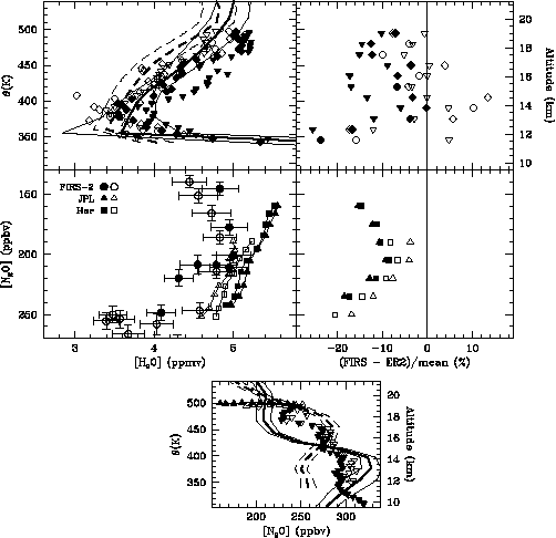
Figure 2.10 Comparison of vertical profiles obtained by the balloon-borne FIRS-2 and in situ instruments on board the NASA ER-2 during flights on 30 April 1997 near Fairbanks, Alaska. Shown in the top left panel are FIRS-2 profiles obtained 250 km North (dashed curve) and Northwest (solid curve) of the ER-2 flight track, as well as in situ measurements of H2O made during ascent (solid symbols) and descent (open symbols). Harvard data are shown as diamonds and JPL as inverted triangles. Average differences between FIRS-2 and in situ measurements of H2O during ascent and descent are shown in the top right panel. Also shown in the middle left panel is a comparison of H2O/N2O correlations for FIRS-2 measurements obtained 250 km North (open circles) and Northwest (solid circles) of the ER-2 flight track with JPL TDL (triangles) and Harvard Lyman-a (squares) measurements made during cruise before (solid symbols) and after sunrise (open symbols). Differences between average FIRS-2 and in situ cruise measurements of H2O are shown in the middle right panel. Also shown is a comparison of FIRS-2 profiles and ALIAS measurements of N2O obtained during cruise (triangles), ascent, and descent (inverted triangles, bottom panel).
Comparison of profiles below 450 K is complicated by the large gradients in H2O caused by propagation of the annual cycle out of the tropics and the difference in horizontal and vertical resolution of the remote sensing and in situ instruments, particularly near the tropopause. Under conditions near 17 km where the comparison is likely to be best, the Harvard and JPL instruments give mixing ratios about 8% larger than FIRS-2.
FIRS-2 and MkIV comparisons
The FIRS-2 and MkIV spectrometers made simultaneous measurements during a balloon flight launched from Ft. Sumner, New Mexico, on 22 May 1994. The gondola was configured to allow FIRS-2 and MkIV to observe 90° apart in azimuth so that FIRS-2 could observe atmospheric thermal emission while MkIV observed the solar absorption spectrum. Early in the flight the gondola was oriented so that FIRS-2 would observe in the same azimuth heading in which MkIV would observe the sunset 7.5 hours later. The stratospheric winds were light during the flight (the balloon drifted less than 50 km between launch and sunset) and so that FIRS-2 and MkIV observed nearly the same airmass. Vertical mixing ratio profiles from this flight are compared in Figure 2.11. Differences between the profiles are generally less than the combined uncertainty of 7%.
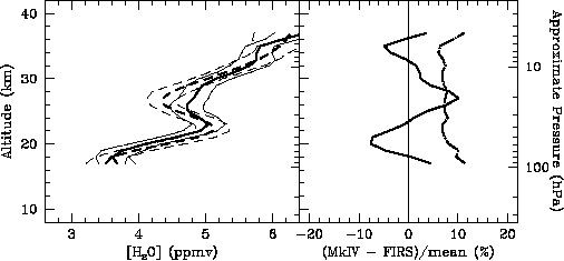
Figure 2.11 Comparison between FIRS-2 (dashed curve) and MkIV (solid curve) profiles obtained during a simultaneous balloon flight on 22-23 May 1994. Individual profiles were derived from observations made 7.5 hours apart in the same azimuth heading (left panel). The difference between the two profiles (solid curve) and combined precision (dot-dash curve) is also shown in the right panel.
2.2.4 Tropospheric measurements
Comparison of Vaisala RS80-A radiosondes and the NOAA-CMDL frostpoint hygrometer
Radiosonde relative humidity (RH) measurements are widely known to be unreliable at cold temperatures. A recent study by Miloshevich et al. [2000] characterised RH measurements from Vaisala RS80-A radiosondes, the most frequently used radiosonde in the world, and developed a correction for the measurements in the temperature range 0°C to -70°C. A data set of simultaneous RH measurements from RS80-A radiosondes and the NOAA-CMDL frostpoint hygrometer (described by Vömel et al. [1995]) was used to derive a statistical correction factor for RS80-A measurements based on the hygrometer measurements. These were operational measurements rather than a controlled intercomparison. The frostpoint hygrometer provides an in situ measurement standard using a technique independent of the operational radiosonde methodology. The calibration uncertainty of the hygrometer is not temperature dependent, and it's response time at cold temperatures is relatively fast. The ratio of each RS80-A and corresponding hygrometer measurement is shown in Figure 2.12 with curves that indicate the mean and standard deviation of the ratio in each 1°C temperature bin. Relative to the hygrometer, the mean RS80-A measurements decrease with decreasing temperature to about 40% of the value of the corresponding hygrometer measurements at -70°C. The RS80-A data are clearly unsuitable for upper tropospheric research studies unless the measurement errors are corrected.
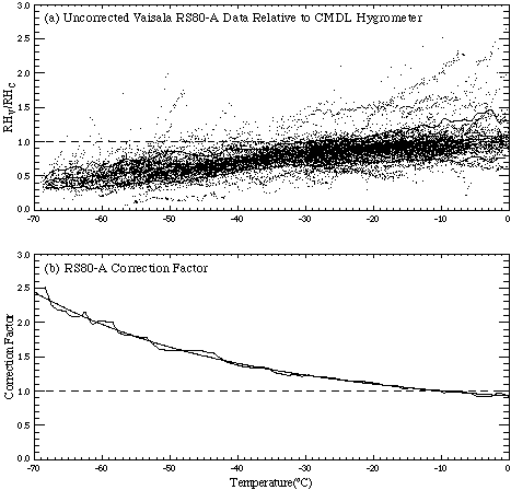
Figure 2.12. (a) Ratio of simultaneous relative humidity measurements from Vaisala RS80-A radiosondes (RHv) and the NOAA-CMDL frostpoint hygrometer (RHc), from eight years of monthly launches at Boulder, Colorado. Curves are the mean and standard deviation (1s) of the ratio in 1° C temperature bins. (b) A statistical correction factor for RS80-A measurements is given by the reciprocal of the mean ratio shown in Panel (a), approximated by the polynomial curve fit shown.
The reciprocal of the mean ratio in Figure 2.12 is the normalisation factor that, when multiplied by RS80-A data, gives corrected RH values that are on average equal to the hygrometer data. This statistical correction factor (curve fit shown in Figure 2.12) accounts for the mean of all sources of RS80-A measurement error combined, as a function of temperature. The magnitude of the correction factor is about 1.1 at -20°C, 1.3 at -35°C, 1.6 at -50°C, 2.0 at -60°C, and 2.4 at -70°C. (The curve fit is not valid outside the temperature range 0°C to -70°C). The fractional uncertainty in the mean of the corrected RS80-A data, when the correction factor is applied statistically to a large data set (such as when constructing a climatology), is estimated to be 0.06 at 0°C and 0.11 at -70°C, which is about 6% RH at ice-saturation at all temperatures. However, the uncertainty when the correction factor is applied to any individual profile is considerably larger, as indicated by the dispersion of the data around the mean in Figure 2.12. This dispersion results from RS80-A measurement errors that are not simply temperature-dependent, but are also sensor-specific or profile-specific. Only the mean value of these errors at a given temperature is considered by this statistical approach.
The RS80-A is subject to several sources of measurement error, and correction of the individual measurement errors is an alternative approach for correcting RS80-A data that is under development. A "temperature-dependence error" is caused by using a linear approximation in the data processing algorithm to represent the actual non-linear temperature dependence of the sensor calibration, and is in general the largest RS80-A measurement error at cold temperatures. The temperature-dependence error depends only on temperature, so it is completely accounted for in the statistical correction. A correction factor for temperature-dependence error has been derived from laboratory measurements conducted at Vaisala. The magnitude of the correction factor is about 1.1 at -35°C, 1.4 at -50°C, 1.8 at -60°C, and 2.5 at -70°C. A "time-lag error" is caused by the exponential increase in the sensor time-constant with decreasing temperature. The time-lag error depends strongly on the rate of change of the ambient RH, so only its average effect at a given temperature is represented in the statistical correction. Simulations show that maximum time-lag errors for conditions when the ambient RH is changing rapidly with altitude are about 5% RH (positive or negative) at -20°C, 15% RH at -40°C, and 30% RH at -60°C; typical time lag errors are considerably less. A correction algorithm for time-lag error is in progress. Chemical contamination of the sensor polymer by non-water molecules, and long-term sensor instability, both lead to dry-bias errors that depend in part on the age of the radiosonde. The magnitude of the combined dry-bias errors is typically 2-6% RH. A moist-bias error of a few percent RH may result from sensor drift under sustained conditions of high ambient RH. Random uncertainty caused by the combination of production variability and uncertainty in the calibration model and the calibration chamber is 4% RH at the 95% confidence level. The RS80-A, like any (unheated) solid-state sensor, is incapable of measuring ice-supersaturation.
It is critical that these corrections be applied only to Vaisala RS80-A data, not to radiosonde RH data in general, and specifically not to Vaisala RS80-H data. The RS80-A and RS80-H both use the Humicap thin-film capacitive sensors, and they differ primarily in the chemical composition and properties of the sensor dielectric material, and in the accuracy of the algorithm for sensor temperature dependence used in the data processing. Although both sensor types are subject to the same general sources of measurement error, the magnitude of each error is highly dependent on the sensor type. This difference is illustrated by the simultaneous RS80-A and RS80-H measurements shown in Figure 2.13. At temperatures colder than --40oC the radiosonde was in a thick orographic cloud where the RH is expected to be near ice-saturation based on independent cloud particle measurements. Most of the difference between the two profiles is due to the difference in their temperature-dependence errors, since the time-lag errors would be minimal after the sensors had been in the cloud at nearly constant RH for 1-2 minutes. It is apparent that the temperature-dependence algorithm for the RS80-H is considerably more accurate than the algorithm for the RS80-A.
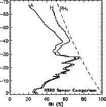
Figure 2.13 Profiles of relative humidity measured simultaneously by Vaisala RS80-A and RS80-H radiosondes. Dashed curve is ice-saturation (RHi).
In conclusion, comparison of relative humidity measurements from Vaisala RS80-A radiosondes using the NOAA-CMDL frostpoint hygrometer as an in situ measurement standard demonstrates that uncorrected RS80-A data are not suitable for upper tropospheric research applications. Correction for well-understood measurement errors substantially improves the accuracy of RS80-A measurements at cold temperatures, probably into the realm of usefulness in the upper troposphere. Further improvement is possible and in progress.
LMD cryogenic frostpoint and LaRC/ARC DLH comparison
An in-flight intercomparison between the aircraft borne LMD cryogenic frostpoint hygrometer and the NASA-LaRC/ARC Diode Laser Hygrometer (DLH) was conducted during the co-ordinated phases of the Pollution from Aircraft Emissions in the North Atlantic Flight Corridor 2 (POLINAT2) European campaign and the Subsonic Assessment Ozone and NOx Experiment (SONEX) U.S. campaign in October 1998. The LMD frostpoint and DLH were flown aboard the DLR Falcon and NASA DC-8 research aircraft, respectively. Good spatial and temporal overlap between both aircraft during two co-ordinated flights provided an excellent opportunity for the intercomparison, which occurred in the upper troposphere between approximately 7 and 10 kilometres.
From the data obtained it has been shown [Vay et al., 2000] that both instruments agreed within 10% over the range of mixing ratios 82 to 900 ppmv. In general, the DLH reported greater water vapour mixing ratios than the frostpoint hygrometer except at the smaller mixing ratios where the best agreement was noted. This may be explained in part by an offset caused by the presence of residual water vapour within the laser head of the DLH discovered during post-mission calibrations. Figure 2.14 is a comparison of the LMD frostpoint and the DLH data for one of the flights. Here the data from both instruments are averaged to 15 seconds to take into account the difference in time response of the DLH (50 ms) and the LMD frostpoint (10 s).
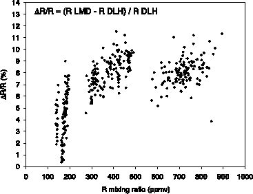
Figure 2.14 Intercomparison between the LMD cryogenic frostpoint hygrometer and the LaRC Diode Laser Hygrometer for the wing tip to wing tip flight on 23 October 1997. Three different altitude legs were sampled at 7.6, 8.9, and 10 km respectively.
In-flight comparison of the MOZAIC humidity device with Lyman-a and LMD frostpoint hygrometer
In Chapter 1 the in-flight uncertainty of the MOZAIC humidity sensing devices (AD-FS2) employed on board five A340 in-service aircraft has been evaluated. From the regular pre- and post flight calibration of each flown sensor, typical 2s uncertainties of ± 5-10% in relative humidity between 10 and 12 km altitude were derived [Helten et al., 1998]. During two dedicated missions with a Fanjet Falcon E research aircraft of the Deutsches Zentrum für Luft- und Raumfahrt (DLR), the in-flight performance of the MOZAIC humidity device was assessed by intercomparison with reference instrumentation.
In-flight comparison, March 1995: Time response and spatial resolution
The first in-flight comparison of the MOZAIC humidity-sensing device against reference instrumentation was conducted in March 1995 with the MOZAIC device mounted aboard the Falcon aircraft [Helten et al., 1998]. As reference instruments for the water vapour concentration measurement, two different types of airborne hygrometers were used: the Jülich Lyman-a fluorescence hygrometer, FISH, with a relative humidity accuracy of ± 5% [Zöger et al., 1999a], and a DLR cryogenic frostpoint hygrometer, with a relative humidity accuracy of ± 10% [Busen and Buck, 1995]. During two comparison flights which took place over Germany, the FISH Lyman-a and the frostpoint hygrometers agreed within their combined uncertainties [Zöger et al., 1999a]. In the middle and upper troposphere, the MOZAIC humidity device agreed to within ± 10% RH (2s -uncertainty level) with the two reference instruments, if averaged over more than one minute. A dry bias of about 10% is indicated for the MOZAIC device. The MOZAIC sensor smoothes the structure in the water vapour that is measured with the reference instruments. This is caused by the response time of the MOZAIC device that increases with decreasing sensor temperature due to the adsorption and diffusion of water molecules into the sensor material [Antikainen and Paukkunen, 1994]. At sensor temperatures of about ?30ºC (the ambient air temperature is below -30ºC) the response time is several minutes. At higher temperatures the MOZAIC instrument tracks fine structures in the humidity field within ± 5-10% RH (2s -uncertainty level).
Based on these comparisons, it was found that the response time of the MOZAIC sensor during ascent and descent is less than 10 seconds near the ground and less than one minute around 9-km altitude. This means that at an ascent/descent rate of the MOZAIC-aircraft of about 8 m/s, the vertical resolution of measured vertical humidity profiles is better than 100 m in the lower troposphere, and approximately 500m in the upper troposphere. At cruise altitude, the response time is about 1-3 minutes. At a horizontal aircraft speed of 250 m/s, the horizontal resolution is about 15-50 km, which is sufficient to record large-scale features in upper tropospheric water vapour.
In-flight comparison, September 1997: MOZAIC versus POLINAT-2
In September 1997, during the European POLINAT-2 (Pollution from Aircraft Emissions in the North Atlantic Flight Corridor) aircraft mission [Schumann et al., 1998], an intercomparison of airborne in situ water vapour measurements was performed between water vapour sensors aboard the Airbus A340 (MOZAIC) and Falcon (POLINAT) aircraft [Helten et al., 1999]. The POLINAT aircraft used the LMD frostpoint hygrometer developed for airborne water vapour mixing ratio measurements [Ovarlez and van Velthoven, 1997]. The intercomparison took place southwest of Ireland on 24 September 1997 at the 239 hPa flight level. The ambient air temperature ranged from -53 to -55ºC. The Falcon approached the flight path of the Airbus at 13°W longitude and followed until 7°W longitude. The Falcon followed the Airbus at a distance of 7-35 km. This corresponds to a time lag increasing from 30s to 160s. The relative humidity measured on the POLINAT aircraft (thin curve) was shifted with respect to the MOZAIC measured relative humidity (thick curve) such that the POLINAT data are for the same longitude as the MOZAIC data (Figure 2.15). The shift was computed using the measured horizontal wind and assuming isobaric transport.
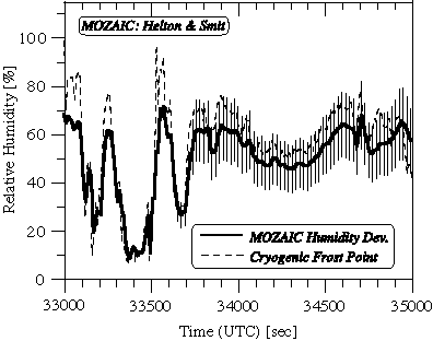
Figure 2.15 Relative humidity measured by the MOZAIC humidity device and the LMD frostpoint hygrometer as a function of flight time during the tropospheric segment of a comparison flight on board the DLR Falcon aircraft in March 1997. The thin vertical lines represent the ± 2s uncertainty levels derived from pre- and post flight calibration of the flown MOZAIC sensor.
The accuracy of the POLINAT water vapour measurements was better than ± 3% [Ovarlez and van Velthoven, 1997]. Figure 2.16 reveals agreement within ± 5% for segment C of the intercomparison where the trajectories of both aircraft where closest. Even mesoscale structures of the water vapour mixing ratio are reproduced. One exception is the strong decrease in water vapour concentration at 8°W longitude, where the values measured by MOZAIC decreased much faster. This occurred in a region with a strong relative humidity gradient, where the time delay between both measurements is a maximum (~160s). Additionally, the POLINAT measurement on its flight back at this position showed a strong change of the water vapour mixing ratio within a short period of time. Therefore, a change in the water vapour distribution could have contributed to the larger deviation. In segment B, where the Falcon flew into a contrail of the Airbus, frostpoint mixing ratios are significantly larger than the MOZAIC measurements. Local increases in mixing ratio of about 3 ppmv are to be expected in aircraft plumes of 100s age [Schumann et al., 1998]. The structures of both measurements in segment A are similar, but the POLINAT values are up to 14% greater than the MOZAIC measurement. This could be partly due to the horizontal water vapour gradient present, since the flight trajectories differ up to 5 km in latitude. The water vapour volume mixing ratio measurements in the range of 80 to 120 ppmv of both instruments differ by less than ± 5%, where the trajectories of both aircraft are very close. The corresponding relative humidity was changing between 50 and 75%. Relative humidity and mixing ratio from MOZAIC and LMD during POLINAT agreed to within 5% for mixing ratios above 80 ppmv. This indicates that the MOZAIC instrument measures upper tropospheric relative humidity and water vapour mixing ratio with an absolute overall accuracy similar to that of the LMD frostpoint hygrometer aircraft sensor.
The results of the two in-flight comparisons of the MOZAIC humidity device with reference instrumentation agree within the 2s -uncertainties of ± 5-10% derived from the individual pre- and post-flight calibration of each flown sensor. It appears that in the upper troposphere at a cruise altitude between 10 and 12 km the MOZAIC humidity device measures relative humidity with an in-flight 2s -uncertainty of ± 5-10%.
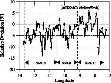
Figure 2.16 Relative differences (MOZAIC-LMD Hygrometer)/LMD Hygrometer in percent obtained during comparison flights between the MOZAIC device on the Airbus aircraft and the LMD frostpoint hygrometer on the DLR Falcon aircraft. Different segments of the flight as described in the text are noted with arrows. The MOZAIC measurement is shifted by 15 seconds opposite to the flight direction to correct for the slower response compared to the LMD frostpoint sensor on the Falcon aircraft.
Comparison of airborne DIAL LIDAR (LASE) with other instruments
The Lidar Atmospheric Sensing Experiment, LASE, uses the DIAL method that provides direct detection of absorption due to water vapour and makes absolute measurements of water vapour profiles without the need for inversion methods. In principle, no field calibration is needed for the LASE measurements, which use the known spectroscopic characteristics of the water vapour absorption lines. Prior to the LASE measurements, very high-resolution laser spectroscopy was conducted for accurate characterisation of water vapour line parameters. The estimated combined error in the water vapour absorption cross-section is ~2-3% in the 720 and 820 nm regions [Grossmann and Browell, 1989a; Grossmann and Browell, 1989b; Ponsardin and Browell, 1997].
Because LASE operates locked to a water vapour line and no wavelength drifts are possible [Browell et al., 1997], no in-flight calibrations of wavelength or linewidth are performed. However, regular checks are done on the ground to ensure proper operation of the LASE system. In addition, to assess the water vapour measurement capability of LASE, a comprehensive LASE Validation Field Experiment was conducted in September 1995 at the NASA Wallops Flight Facility. LASE measurements were intercompared with a number of in situ and remote sensors from the ground and other aircraft [Browell et al., 1997]. These sensors included radiosondes, airborne dew point and frostpoint hygrometers, and remote LIDAR water vapour measurements from the ground and aircraft. An example of an intercomparison of water vapour profile measurements is given in Figure 2.17, illustrating the sensitivity and accuracy of the LASE measurements as shown in the agreement with other sensors. The Vaisala sondes appear to underestimate water vapour measurements compared to LASE in the upper-troposphere. This feature is consistent with the known dry bias of Vaisala sondes [Clough et al., 1996]. For the entire field experiment, 39 profile comparisons were made when the time difference was less than 30 minutes. The mean of the average profile differences was less than 2% with standard deviations less than 10% [Browell et al., 1997]. When small altitude shifts (? 120 m, well within the uncertainty in the height determination from the radiosondes) are used to align prominent atmospheric features in the comparison profiles, then standard deviations decrease to 7%. In order to account for horizontal variability, comparisons were also performed with the in situ aircraft flying at several different constant altitudes. An average of the 65 comparisons showed a mean difference of 1.6% with a standard deviation of 6%. When compared with all the water vapour measurements acquired during this experiment, LASE water vapour measurements were found to have an accuracy of better than 6% or 0.01 g/kg whichever is larger, across the entire troposphere [Browell et al., 1997].
LASE has been operated from the NASA ER-2, DC-8, and P-3 aircraft, and has participated in five major field experiments during 1995-1999 as discussed in Chapter 1. During each of these field experiments the LASE water vapour measurement accuracy has been verified by comparison with other remote and in situ water vapour sensors.
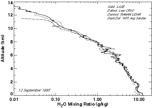
Figure 2.17 Comparison of LASE measurements with the Lear Jet cryogenic hygrometer, NASA Goddard Raman LIDAR, and Vaisala radiosonde measurements made near the Wallops Flight Facility on 12 September 1995.
Raman LIDAR and H-Humicap sensor comparisons
The comparison of water vapour mixing ratio measured by the OHP LIDAR and radiosondes (H-Humicap, RS80) launched simultaneously at the same site reveals a dispersion of 2% and no significant bias (<1%) up to 9 km for 20 coincident measurements. Above 9 km, the water vapour density measured with the LIDAR exceeds radiosonde measurements by 2-5%. This is probably due to temperature dependence and hysteresis effects of the H-Humicap sensor. When the comparison is performed as a function of mixing ratio values, H-Humicap underestimates water vapour (2%) for densities larger than 0.001 g/g of dry air and overestimates water vapour (2-5%) for densities smaller than 0.0001 g/g of dry air. This effect leads to a discrepancy in the water vapour distribution observed with the two instruments mainly at the extremes of the distribution. It also appears that the H-Humicap sensor has a bias (5%) for temperatures lower than 220-230 K, corresponding to typical upper tropospheric conditions.