Previous: Theoretical considerations Next: Results and discussion Up: Ext. Abst.

Data and Methodology

N values for each l pair, and total O₃ values, measured using Dobson O₃ Spectrophotometer number 18, located at Chiromo campus, University of Nairobi, Kenya, were collected. Only those data obtained during clear conditions were considered [that is, Direct Sun (DS) measurements ].

Monthly standard lamp tests, ensured accurate measurements.

(i). Evaluation of I_A, I_C and I_D

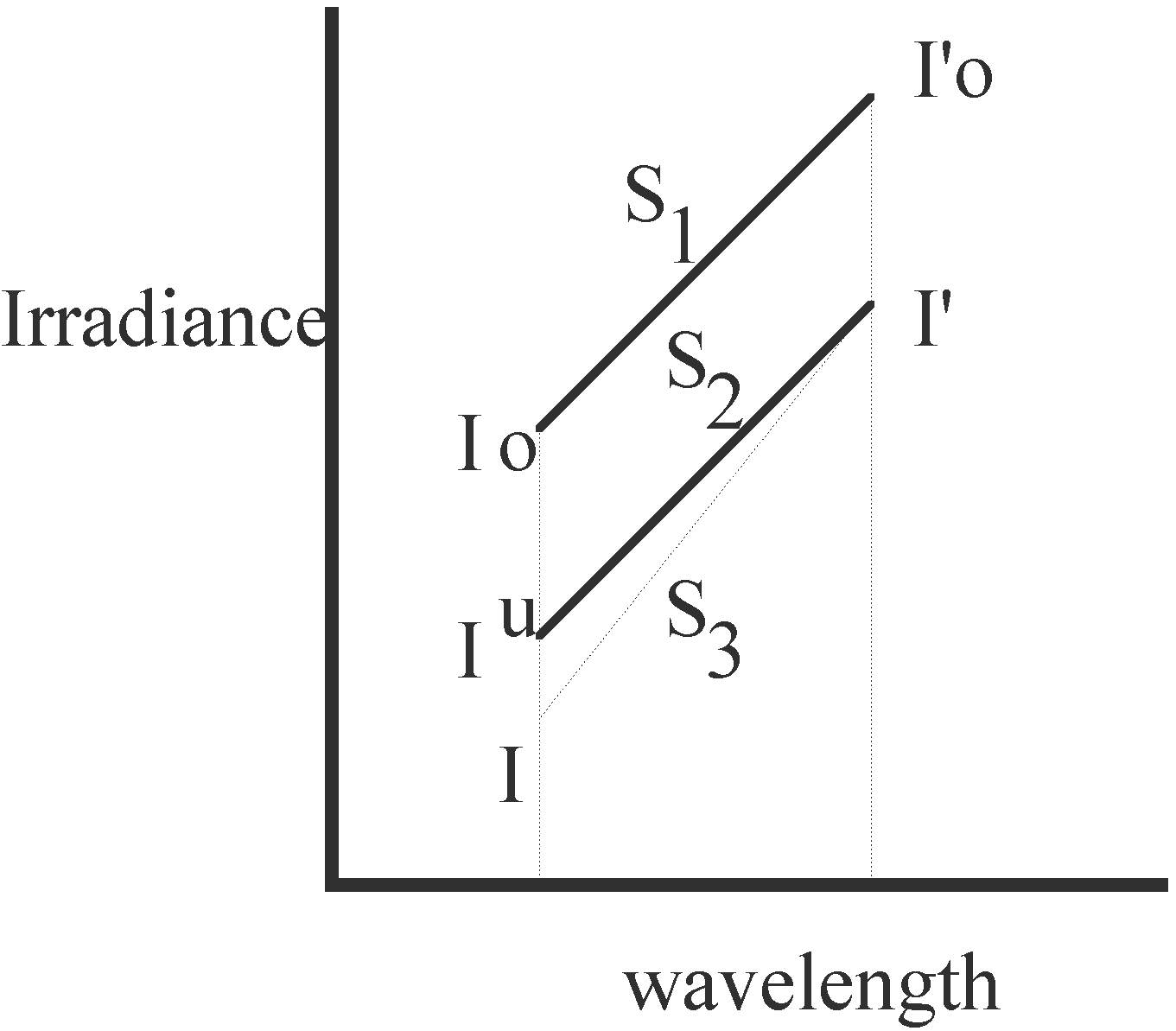
Assuming that a pair of l s e.g. A is affected by the same attenuation, except for O₃ absorption, the irradiances I_A, I_C and I_D are deduced by assuming a linear relationship between irradiance at top of atmosphere and the irradiance reaching the surface (assuming no O₃ absorption occurs). Figure 1 shows that relationship.

Figure 1: The relative attenuation of Dobson O₃ Spectrophotometer l pair

where I _o, I’ _o = long and short l Extra terrestrial (ET) spectral irradiance, I^u = short wave radiation if no O₃ absorption were to occur, I = actual radiation on the surface, I ’ = long wave radiation. From figure 1, linear attenuation implies that

...........…………………………..…........(5)

where l _A and l _A’ are the l s corresponding to I _o and I _o’, respectively. a = is known Frohlich (1986). Equation 2 can be rewritten as ..………………….....(6)

where . Total O₃ is theoretically inversely related to I/I’ . Thus, regressing I/I’ against O₃ we obtain

.......………………………………….................................(7)

b= (i.e. value of when O₃= 0). Effectively, in this study, therefore, a monthly value of b is computed after regressing on O₃ for a given set of observations in a given month. By considering measurements taken within 30 minutes time interval the effect of diurnal UV variability is minimised. This time interval is adopted in this study. After determination of b, by considering equation (5) we have,

.........……………………………………….....(8)

then ...........………………………………………………….......(9)

where a_o =(I’ _o - I _o), and b are evaluated using ET solar spectral irradiance values for the respective l s obtained from Frohlich (1986).

Assuming a mean value of I’ for the respective period (in this case a month) under consideration, I can then be computed from equation (9).

(ii) Method of analysis

Direct sun (DS) total ozone measurements for the periods January 1993 to January 1998 were collected. This way, the effect of clouds was eliminated. Frequency analysis of observation times of the measurements for the period 1993 to 1998 was performed. Only the months of January and September were considered, representing minimum and maximum ozone occurrence periods, respectively, over Nairobi (Muthama, 1989). By considering time intervals of 30 minutes in order to eliminate diurnal UV variability, the most frequent times of ozone observations in January were found to be at the time intervals 7:30 -8:00 and 11:30-12:00. The 11:30-12:00 time interval was also found to highly frequent in September and it was selected for analysis. The September 7:30-8:00 interval had only 3 data points and it was thus not included in the analysis.

The N values recorded from the instrument, for January and September, were utilised to compute ratios using equation (6). The ratios, together with ozone values, were then fitted into a linear distribution fit. Such fit was preferred on the basis of the assumption that the two wavelengths under consideration are relatively affected by the same attenuation, apart from the ozone absorption. The b values from equation(7), for the A, C, and D wavelength pairs were computed. By equation (9), I’ values for January and September were obtained for both the two time intervals.