![]() (2)
(2)
Meteorological Observatory of Moscow State University, Russia
FIGURES
Abstract
1. Introduction
The cloudiness and ozone are the main factors that change biologically
active UVB irradiance coming to the ground. During the last years
a lot of efforts were done to organize ground UVB network. But
the period of continuous UVB observations is not very long and
for most stations does not exceed a decade. A distinct growth
of total ozone amount observed during the last years may be responsible
for increase in UVB irradiance, but possible changes in cloud
properties and amount may compensate or enhance the changes in
UVB irradiance due to total ozone increase. Therefore it was interesting
to study UVB variations due to ozone and cloudiness changes separately
in order to reveal the significance of each factor and to define
the geographical regions where the interannual variability of
UVB irradiance is determined mainly by this or that parameter.
Using historical records of cloud observations and long-term ground
measurements of total ozone amount as well as satellite data we
try to estimate the long-term UV irradiance variations in different
geographical regions.
2. Data and method description
Following the RAF ideology described in [Booth and Madronich,
1994] which is based on the existence of power law dependence
between the UVB irradiance and total ozone we calculated UVB relative
changes due to ozone using the following equation:
Ai(Xi)=X i RAF/Xmean RAF (1)
where RAF=-1.1 for CIE erythemally weighted (EW) irradiance and RAF=-2.1 for Setlow weighted irradiance [Madronich et al., 1998].
To estimate the cloud effects we use the CQg parameter which can be evaluated using only visual cloud observations
and precalculated dependence of UV transmittance on different
cloud amount [Chubarova, 1998]. According to Chubarova and Nezval’
[2000] the resulting UV transmittance by clouds (CQg) can be written as:
![]() (2)
(2)
where Pi(N,Nl) is the frequency of low level cloud amount (Nl) with different amounts of total cloudiness (N); Pi(10,Nl) is the frequency when total cloud amount is equal to 10, always corresponding to overcast conditions, but with different amount of low level clouds; CQ(Nl) is the UV transmittance by low cloudiness; CQup is the UV transmittance by upper level clouds under overcast conditions.
In our previous study [Chubarova and Nezval’, 2000] it was shown that speaking of year-to-year variations in UVB irradiance, the changes in total ozone and in CQg cloud parameter play the main role if compare with variations in aerosol and in cloud optical thickness. This fact enables us to calculate the changes in UVB due to cloudiness and ozone when there is no any radiation measurements and, hence, to reconstruct the historically changes in UVB irradiance. For calculating the CQg parameter we use 3 and 6 hourly cloud amount observations from 19 meteorological stations located in different regions of the former Soviet Union since the middle of the 30s which were available from cdiac.esd.ornl.gov/epubs/ndp/ndp048. We also use the observations from several ground ozone stations stored in WOUDC archive (www.tor.ec.gc.ca/woudc/data/). The longest period of ground ozone observation covers 1926-1998 (Arosa, Switserland, [Staehelin et al., 1998]).
We also used TOMS ozone and UV Reflectivity at 380 nm (R380) data,
which were available from http://jwocky.gsfc.nasa.gov/ for the
periods of 1979-1992 and 1997-1999. R380 was used to estimate
the cloud-aerosol transmittance in the atmosphere according to
the method proposed in [Eck et al., 1995]:
CQ TOMS=1 - ( R380 –Rs )/( 1 - 2 Rs), when R380£ 0.5 (3)
CQ TOMS=1 - R380 , when R380>0.5 (4)
where Rs is the surface reflectivity. We consider Rs=0.03.
3. Validation of the method for retrieving UV irradiance variations
The proposed method was verified on the base of two datasets with a lot of ancillary information: broadband UVB measurements in Moscow (Meteorological Observatory of Moscow State University, MO MSU) and NSF UV spectroradiometer network data.
3.1 Validation according to Moscow broadband UVB data.
During 1994-1996 period the EW irradiance was measured by temperature stabilized Biometer 501 with a solar angle dependent calibration factor obtained in Finland in 1995 during WMO/STUK intercomparisons. Since 1999 the UVB measurements were resumed by UVB-1 Pyranometer (Yankee Environmental Systems Inc.) which has been checked at Colorado UV facility which is guided by the joint efforts of Natural Resource Ecology Laboratory of Colorado State University and NOAA. The calibration of UVB-1 signals in the units of EW irradiance was implemented using the method proposed in Lantz [1999]. Fig.1 shows a good agreement between the estimated and measured monthly means EW irradiance in snow-free conditions for both periods; correlation coefficient comprises R2=73%.
We also use TOMS data to compare the retrievals of EW irradiance over Moscow. Fig.2 shows a coincidence between the EW irradiance obtained from satellite and by using the proposed method. R2=87% if we use all ancillary data including the aerosol and cloud optical thickness to retrieve EW irradiance (see violet line in Fig.2) and R2=78% if we use only ozone and CQg parameter (see black line with squares). A good agreement in Fig. 1 and in Fig.2, i.e. between the measured EW irradiance and the EW estimated from ground and satellite data may be explained by a good agreement in input parameters –cloudiness and ozone. It is known that there is a good agreement between ground and satellite retrievals of total ozone. That is why we focused on the examination of cloud parameter. We used the data of 19 stations in different geographical areas to check the similarity in interannual variations of CQg parameter, total cloud amount (NA) and the CQ obtained from satellite. Fig.3 illustrates these comparisons over different geographical regions. There is a good agreement in relative year-to-year changes between CQ TOMS and ground CQg values, but CQ TOMS are systematically 5-20% lower due to aerosol attenuation, which is considered together with cloud attenuation according to the TOMS algorithm. Table 1 shows determination coefficients, R2, which are calculated between CQ TOMS and NA, between CQ TOMS and CQg values. We received a better agreement with the CQg values and in some cases the difference in R2 is very high due to prevailing thin upper cloudiness in several regions, which has been accounted for while calculating of CQg. On the other hand, a good correlation between interannual variation of CQ TOMS and CQg obtained as a weighted cloud amount parameter is an evidence, that it is cloud amount variation that plays a main role in CQ TOMS variability while variations in aerosol and cloud optical thickness make up only a few percents (R2 =83% if we add the effects of cloud optical thickness and R2 =87% if we add aerosol fluctuations (see Table 1)). At the same time we understand that other atmospheric factors may be of more importance if day-to-day variability of CQ TOMS values are discussed.
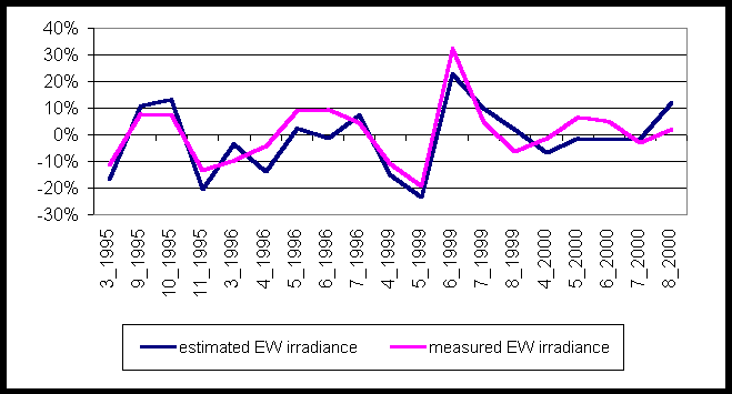
Fig.1. Measured and estimated EW irradiance variability. Snow-free conditions,
Moscow 1995-2000.
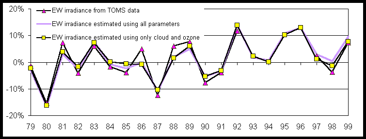
Fig.2. Comparisons between EW irradiance variations obtained from TOMS
data and estimated using ground ancillary information. May-September
period, Moscow.
Table 1
|
PARAMETER |
|
||
|
Olenek j =68.5N l =112.4E |
Skovorodino j =54N l =123.97E |
Moscow j =55.7N l =37.5E |
|
| Total cloud amount, NA |
|
|
|
| CQg |
|
|
|
| CQg + accounting the cloud optical thickness |
|
||
| CQg + accounting all available parameters |
|
||
3.2 Validation according to NSF spectral dataset.
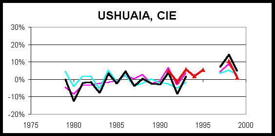
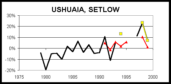
In order to compare UVB retrievals in other geographical conditions we used the NSF spectral dataset which is supported with a lot of ancillary information and is available via bsimail.biospherical.com/nsf. The analysis was made for CIE EW irradiance and for Setlow dose in snow free conditions over Ushuaia, San Diego and Barrow sites. Fig.3 illustrates a good agreement in estimated and measured EW irradiance variability (R2=89% for Ushuaia and R2=82% for San Diego). For Setlow dose the correlation is less (R2 is about 60%) presumably due to more sensitivity to other atmospheric parameters. Figure 4 illustrates an agreement between interannual variations in CIE EW irradiance and in Setlow dose as well as distinct upward trends obtained from both TOMS data and the NSF measurements mainly due to ozone loss over Ushuaia. The effect of ozone loss was enhanced by growth in CQ transmittance during the last years (see Fig.4a). There is also a good agreement in TOMS and NSF data for Barrow and San Diego sites. The analysis of year-to-year variations in EW irradiance and Setlow doze for these sites has not revealed any trend.
a/ b/
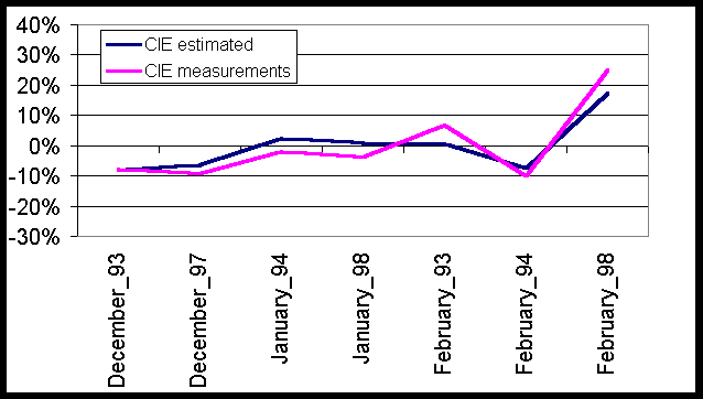
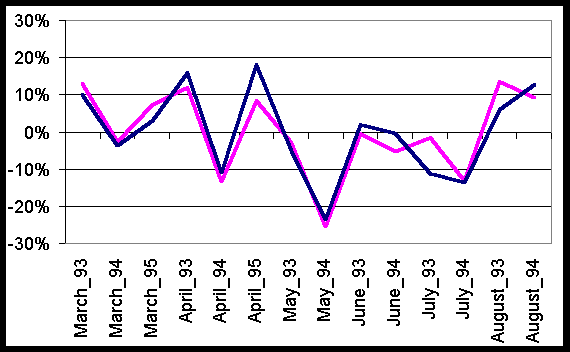
Fig.3. Measured and calculated variability of CIE EW irradiance in Ushuaia
(a, austral summer) and in San Diego (b, boreal warm period).
a/ b/
c/ d/
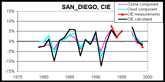
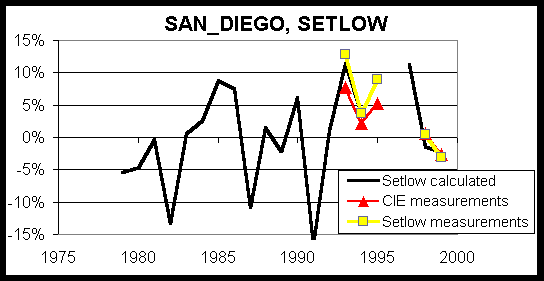
Fig. 4. Variability of biologically active irradiance according to NSF measurements and TOMS data (in black) in Ushuaia (a,b) and San Diego( c,d). CIE EW irradiance is shown by red line with triangles (a,c) and Setlow weighted irradiance - by yellow line with squares (b,d). EW variability due to cloudiness (blue line) and due to ozone variations (pink line) are shown in 5a,c. Summer periods.
4. EW irradiance variations due to ozone and cloudiness
Using the historical data of cloud observations as well as ground ozone measurements we reconstructed variations in EW irradiance due to clouds and ozone in different geographical regions during warm period. Fig.5 illustrates variability in EW irradiance inferred from ground and satellite measurements for several Eurasian sites since the 1920-30s. It is clearly seen that there are different tendencies in CQg variations at different sites. We observe a significant CQg growth (about 10%) at the end of 30s over the Northern part of Eastern Europe, a strong CQg decrease over continental region of Western Siberia at the end of 40s, and in the 50s -over the Monsoon Far East area, where the CQg growth (higher than 10%) was observed in the middle of 80s. EW irradiance variations due to ozone changes have slightly less amplitude at the sites analyzed. But even over Arosa, where the ground ozone measurements were available since the middle of 1920x , the maximum changes of EW irradiance due to ozone comprise about ± 7%. It is necessary to emphasize that in several regions interannual changes in ozone and cloudiness are correlated (i.e. R2>30% for Arosa, Nikolaevsk-na-Amure, Irkutsk, etc): i.e. the minimum in ozone values corresponds to the higher cloud transmittance. The same picture was observed over San Diego (R2 >55%) and, to some extent, over Ushuaia.(see Fig 4). This effect may significantly enhance the EW growth in conditions of ozone loss.
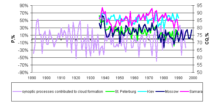
In order to reveal the main cause of the cloud fluctuation we analyzed relative changes in CQg for the sites within the Atlantic Continental region of Eastern Europe together with the examination of synoptic processes according to classification of Klimenko [1999], which has been developed for this region. The classification is based on the revealing of typical cyclone and anticyclone trajectories at the Russian Plane and was applied for 100 year period. Fig. 6 shows interannual variation of the processes with cyclonic origin (P), which contribute to cloud formation and relative CQg changes within the analyzed territory. The correlation coefficients between the CQg at different sites are significant at 95% level and lie in the range of r=0.4-0.65, while there is strong inverse correlation of CQg against P variability with r =-0.68. Therefore we may reliably reveal the periods of relatively high CQg values in the past which cover the middle of 30s and the end of 60s due to attenuation of cyclonic activity over the Russian Plane. At the same time after 1976 there was a significant decreasing of CQg values almost at all sites over this region. The application of Fourier spectral analysis has revealed the periods of approximately 2, 4 and 9 years in variability of CQg at three sites, except Samara, similar to those in variations of P processes (Fig. 6b). The Samara peculiarity can be explained by its boundary location at the eastern part of the Russian Plane.
In order to compare the mean cloud and ozone effects on EW irradiance we use the following parameters:
Vcl=2s cl / CQ, (5)
VX=2s (Ai(X)) / XmeanRAF (6)
D=Vcl-VX (7)
where Ai(X ) was determined in (1), s cl and s (Ai(X)) are the standard deviations of CQ transmittance and A(X). Thereby, Vcl and VX characterize the normalized EW irradiance variations due to cloudiness and ozone within a 95% significant interval. D is the difference between the cloud and ozone effects on EW irradiance.
Fig.7 shows the EW variations due to ozone and cloud changes obtained from satellite and ground observations for different time scales over Eurasia. For most sites the EW variability due to ozone evaluated from long-term ground measurements (VX ) lies within few percents with VX obtained from TOMS. The maximum VX is observed for ground ozone measurements and comprises 10-11%. EW changes due to cloud effects retrieved from ground cloud observations since the middle of 30s can reach 14-16%, and are mainly in agreement with TOMS Vcl values obtained for much less period. The sites with positive UV trend can be noticed over Southern Europe (42-44° N, the Mediterranean), over the local areas in Central Asia, where the effects of ozone and cloudiness are comparable, and the areas in Central Europe (50-52° N), which are characterized by high cloud variations. The observed EW increase over Eurasia is the combination of variability in ozone and cloudiness impacts.
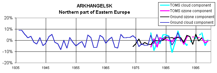
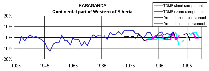
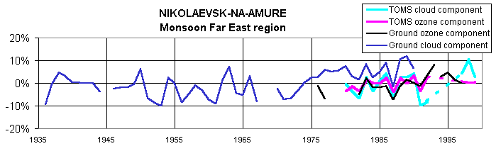
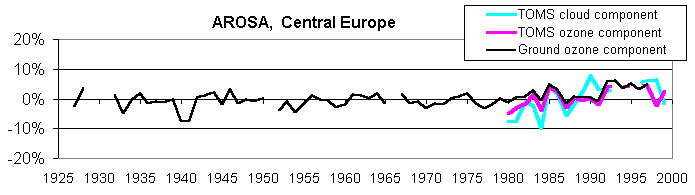
Fig.5. Interannual EW variability due to cloud and ozone component obtained from ground and satellite measurements in different geographical regions. May-September period
a/
b/
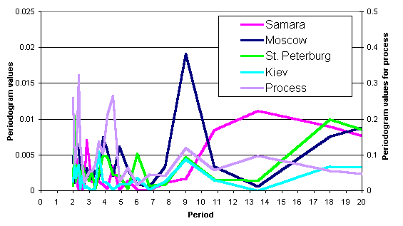
Fig.6. a/ Interannual variations in cloud transmittance (CQg ) and in synoptic process responsible for cloud formation (P) according to [Klimenko, 1999] within the Atlantic- continental region of Eastern Europe, in percents; b/ Periodogram obtained by Fourier (spectral) analysis. May-September. Periodogram was set for the 1936-1990 period.
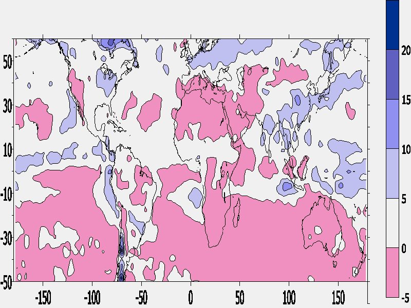
Fig. 8 shows the difference D=Vcl-VX between the effects of clouds and ozone on EW variability. The
cloud effects on EW variability can be significantly higher than
ozone effects, but this phenomenon takes place only in local areas:
over the Northern part of Europe, Northern Canada, the South-Eastern
monsoon regions of Asia, etc., which are characterized by temporally
erratic but intensive circulation processes. On the whole, the
effects of ozone and cloud on EW variability are comparable and
lie within ± 5% for most of the Earth’s territory. The effects of ozone slightly
dominate in Southern Hemisphere(D<0%). During May-September period they also prevail over Northern
Africa, Mediterranean region, and local areas inside the continents
(see Fig.8a) covering low latitude zones, where EW doses are large
(see the distribution of EW irradiance in Fig.7). During November-March
period the area of prevailing ozone effects on EW irradiance decreases
but still it covers a large territory.
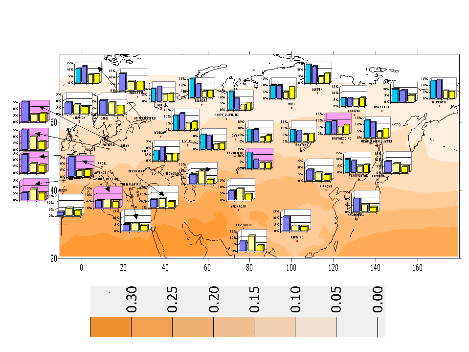
Fig.7. EW irradiance over Eurasia (summer solstice, W/m2 ) and its
changes due to cloud variability obtained from ground (light blue
columns), from TOMS (blue columns) and due to ozone variations
inferred from ground (light yellow columns), from TOMS (yellow
columns). The sites with significant positive trend according
to TOMS data are marked with pink background. May-September period.
a/
b/
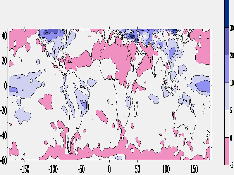
Fig. 8. Spatial distribution of D=Vcl-VX for comparison in effects of cloudiness and ozone variations on EW irradiance. May-September (a) and November-March periods(b). Negative values denote the areas with prevailing changes in EW irradiance due to ozone and positive values– due to cloud effects.
4. Conclusions
Acknowledgements
The author would like to express her gratitude to Natalia Uliumdzhieva,
Alla Yurova and Anna Suslova for their technical help. The author
wish to thank the personnel who have prepared the dataset of NSF
UV spectroradiometer network, the ozone and UV database of World
Ozone Ultraviolet Radiation Data Centre, TOMS database and the
database of CDIAC Data Center, which were used in this study.
References
Booth C.R. and S. Madronich, 1994: Radiation amplification factors: improved formulations accounts for large increases in ultraviolet radiation associated with antarctic ozone depletion // Ultraviolet radiation in Antarctica: measurements and biological effects. Washington, DC, 39-42.
Chubarova, N.Ye., 1998: Ultraviolet radiation under broken cloud conditions as inferred from many-year ground-based observations, Izvestiya. Atmospheric and Oceanic Physics, 34, 131-135.
Chubarova N. and Ye. Nezval', 2000: Thirty year variability of UV irradiance in Moscow, Journal of the Geophysical Research, Atmospheres, 105, 12529-12539.
Eck T.F., Bhartia P.K., Kerr J.B.,1995: Satellite estimation of spectral surface UV irradiance using TOMS derived total ozone and UV reflectivity. J.Geophys.Res.Letters. v.22, ? 5, 611-614.
Klimenko L.V., 1999: Atmospheric processes at the Eastern European Plane for the last 100 years. Moscow State University Publishing House, pp. 127.( In Russian)
Lantz, K., et al., 1999: Methodology for deriving clear-sky erhtyemal calibration factors for UV broadband radiometers of the US Central Calibration Facility, J. Atmos. Ocean. Tech., 16, 1736-1752.
Madronich S., R.L.McKenzie, L.O.Bjorn, M.M. Caldwell, 1998: Changes in biologically active ultraviolet radiation reaching the Earth’s surface. Journal of Photochemistry and Photobiology B: Biology 46, 5-19.
Staehelin J., et al., 1998: Total ozone series at Arosa (Switzerland): Homogenization and data comparison. Journal of the Geophysical Research, D5, 5827-5841.
Back to
| Session 1 : Stratospheric Processes and their Role in Climate | Session 2 : Stratospheric Indicators of Climate Change |
| Session 3 : Modelling and Diagnosis of Stratospheric Effects on Climate | Session 4 : UV Observations and Modelling |
| AuthorData | |
| Home Page | |