Previous: Lidar and SAGE II Measurement Next: Conclusions Up:Ext. Abst.
3. Discussion
Figure 1 shows the daily IBC mean values of the space coincident SAGE II and lidar mensurements. It covers the period before and after Mt. Pinatubo. Also lidar measurements taken during the Mt. Pinatubo decay period are included.
The pre-Pinatubo lidar IBC have a mean IBC value of 1.52x10⁻⁴ sr-1 and the post-Pinatubo IBC mean value is 2.71x10⁻⁴ sr-1. The apparent increase in the IBC is explained by the presence, during the years 1996 and 1997, of several IBC values higher than the previous ones reached during 1995. Reports from lidars at Mauna Loa (19.5°N, 155.6°W) and at Garmisch-Partenkirchen (47.5°N, 11.0°E) show the presence of aerosols layers in the stratosphere from unknow origin (GVN, 1996;1997). Also increased aerosol optical thickness was measured during that period at two sites: Seguin, Texas, and San Diego, California Those high IBC values were also reported at (Mims et al., 1996).
In general the lidar IBC mean values for both periods are in the order of magnitude reported from Mauna Loa (Barnes and Hofmann, 1997) and from Heffei (Hu, 1998), both tropical stations.
The SAGE II measurements for the same pre and post-Pinatubo periods covered by lidar show a mean IBC value of 1.44x10⁻⁴ sr-1 before the Pinatubo and 1.26x10⁻⁴ sr-1 after. There is a good agreement between the mean IBC values from lidar and SAGE II for the pre-Pinatubo period. For the second period the agreement is not so good. Comparatively, only few of the SAGE II measurements show the relative high IBC values, measured by lidar. A possible explanation is related to the SAGE II sampling features. In the tropical region the grid associated with the space sampling is around 24° in longitude by around 5° in latitude. And the time gap between consecutives SAGE II sampling of the same region of the earth is around six weeks. It means that aerosol clouds within such space dimensions and within that time frame could or could not be measured by chance. Ground based lidars sample always the same point of the earth with a commom time frame of around one week under background conditions. That is one of the features which makes lidar an satellites valuable complementary instruments.
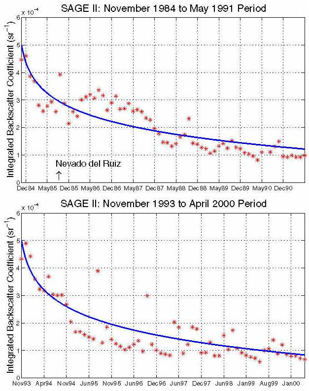
In the Figure 2 the monthly mean IBC values from SAGE II are shown. Both for El Chichon and Pinatubo the period selected cover from around two and half years after the eruption to aproximately
Figure 2. Monthly mean IBC values from SAGE II. Pre-Pinatubo (1984 - 1991) and post-Pinatubo (1993 - 2000).
seven years later. One clear feature is the presence of a seasonal cycle in the IBC, as it had been reported from global analysis of SAGE II data under background conditions (Thomason et al., 1997). Also exponential adjustment for both periods are shown. The decay rate is similar for the post-El Chichón and post-Pinatubo. The e-folding decay period was around 24 months. Additionaly in the case of the 1984 - 1991 period we can see the Nevado del Ruiz (September 11, 1985) eruption clearly superimposed over the decay trend after the El Chichón eruption.
The SAGE II IBC average for the two years before the Pinatubo has a value of 1.138x10⁻⁴ sr-1. In comparison the IBC average for the last two years in the record (May 1998 to April 2000) was 0.976x10⁻⁴ sr-1. The lower IBC value presently is also visible from figures 1 and 2. This result agree with reports that a lower background condition have been reached ultimately (Jager et al., 1998).
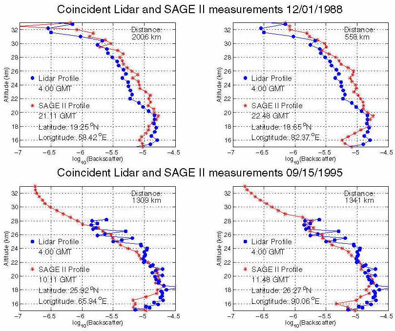
Figure 3. Coincident Lidar and SAGE II backscattering profiles.
The Figure 3 shows, on top, coincident lidar and SAGE II backscattering profiles for December 1st 1988. It consists of one lidar profile and two consecutive SAGE II profiles measured at distances around 500 Km and 2000 Km. Despite the big differences in distance between the SAGE II profiles and the lidar site there are not so big differences. This feature could be attributed to the homogeneity of the stratospheric aerosols under background conditions. On the bottom coincident measurements for September 15th 1995 are shown, in this case both SAGE II profiles are at around the same distance. No big differences are found.