Previous: Introduction Next: Annular Modes in the surface pressure Up: Ext. Abst.
Model description
The Kühlungsborn Mechanistic general Circulation Model (KMCM)
(Becker and Schmitz, 2001) is a dry idealized GCM. The model is
run at moderate resolution with triangular truncation at wavenumber
29 in the horizontal and 24 hybrid levels, up to 0.3 hPa. Temperature
relaxation parametrizes the radiation. The relaxation time is
16 days and drops down to 4 days at the upper rim. All simulations
are ``perpetual January''. In the troposphere, relaxation temperature
1![]() corresponds to observational temperature with increased meridional
gradients. In the stratosphere
corresponds to observational temperature with increased meridional
gradients. In the stratosphere ![]() is related to the radiatively determined state.
is related to the radiatively determined state.
In order to examine the influence of different stationary wave
forcing mechanisms, KMCM yields the possibility to turn them on
or off independently. These mechanisms are world orography (![]() ) as well as additional diabatic heating in the deep tropics (
) as well as additional diabatic heating in the deep tropics (![]() ) and middle latitudes (
) and middle latitudes (![]() ):
):
| (1) |
The first term on the l.h.s. is used to mimic convective heating
in the tropics. The second term describes self-induced condensational
heating in middle latitudes in order to mimic land-sea heating
contrasts. It depends linearly on the pressure velocity ![]() and is only active for rising motions due to the Heavyside function
and is only active for rising motions due to the Heavyside function
![]() .
. ![]() and
and ![]() are prescribed functions of longitude, latitude and pressure
(Becker and Schmitz, 2001, their Fig. 2). For a more detailed
model description, including turbulent boundary layer mixing and
definition of the surface temperature, the reader is referred
to Becker and Schmitz (2001).
are prescribed functions of longitude, latitude and pressure
(Becker and Schmitz, 2001, their Fig. 2). For a more detailed
model description, including turbulent boundary layer mixing and
definition of the surface temperature, the reader is referred
to Becker and Schmitz (2001).
The nomenclature of the model runs consists of the three abbrevations
for the forcing mechanisms. By writing them in brackets or as
function of longitude ![]() it is indicated whether the zonal-mean or the longitude-dependent
field is included. Starting from the rotationally invariant reference
run
it is indicated whether the zonal-mean or the longitude-dependent
field is included. Starting from the rotationally invariant reference
run
![]() , orographic (run
, orographic (run
![]() ), midlatitudinal (run
), midlatitudinal (run
![]() ) and tropical thermal forcing of stationary waves(run
) and tropical thermal forcing of stationary waves(run
![]() ) are added and can be combined with each other (e.g. run
) are added and can be combined with each other (e.g. run
![]() ). All mechanisms are present in run
). All mechanisms are present in run
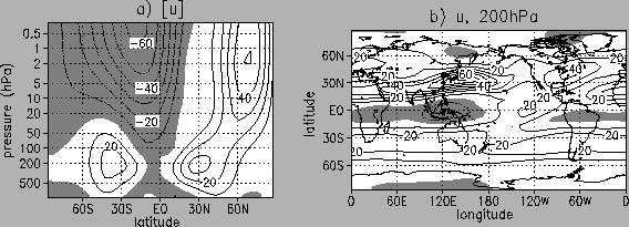
![]() , that generates a realistic mean state of the atmosphere (Fig. 1). The length of each model run is 1801 days.
, that generates a realistic mean state of the atmosphere (Fig. 1). The length of each model run is 1801 days.
Prior to the EOF analysis the model data was smoothed with a binomial
30-day low-pass filter and weighted with the square root of cosine
latitude. The low-pass filter reduced each data set by 128 days.
All EOFs are calculated for the northern hemisphere (![]() N to
N to ![]() N). One-point correlation maps are used for comparison.
N). One-point correlation maps are used for comparison.
 |