Previous: Data Next: Summary Up: Ext. Abst.

4. Results

4.1. NO₂

4.1.1. Seasonal behaviour of NO₂

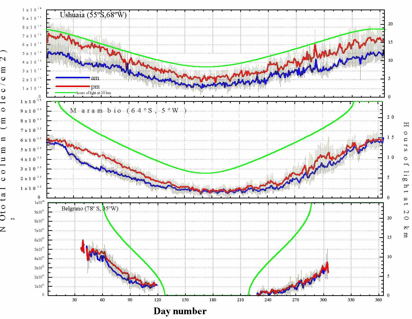
Figure 1. Seasonal wave of the NO₂ column in Ushuaia,Marambio and Belgrano.

Accumulated data provide a picture of the seasonal wave of the NO₂ column (figure 1). Ushuaia displays a seasonality in phase with the hours of light (green line) available at an altitude of 20 km. AM (PM) values range from 1.2x10¹⁵ (2.1x10¹⁵) molec/cm² in winter solstice to 5x10¹⁵ (7x10¹⁵) molec/cm² in summer solstice, with a moderate interannual variability (15-20%). In Marambio the NO₂ minimum (0.7-0.8x10¹⁵ molec/cm²) extends toward the spring since no HNO₃ is available to rebuild the NOx. The recovery starts in mid August; two month delayed from what could be expected from pure photochemistry. At that period there are already 9-10 hours of light at 20 km. It is worthwhile to note that at Marambio latitude, mid-winter light at 20 km is 6.5 hours and more at higher levels. The denitrification is not complete at all altitudes since minima temperatures do not drop much of the theoretical PSC formation. Occasionally PSCs might result from synoptic scale cooling dynamically induced processes at the Antarctic Peninsula range as occur in the Northern Hemisphere across the Scandinavia range (Fricke et al. 1998)

In summer, when the stratosphere is illuminated 24h/day, the NO₂ column stabilises at 6x10¹⁵ molec/cm² since all NOy has already been converted to NOx, and poleward transport is inhibited. The same situation is observed in autumn above Belgrano with 5x10¹⁵ molec/cm². After the polar night, however, there is no increase of the background values (below 4x10¹⁴ molec/cm², instrumental threshold) for almost one month. As for Marambio, increase occurs when the light at 20 km is over 10 hours/day. At the end of the observational period the NO₂ column is still increasing, since the stratosphere is at this time illuminated 24h/day, and the vortex is still strong. NO₂ must come from downwelling HNO₃ reservoir

4.1.2. Interannual variability. SLIMCAT comparison.

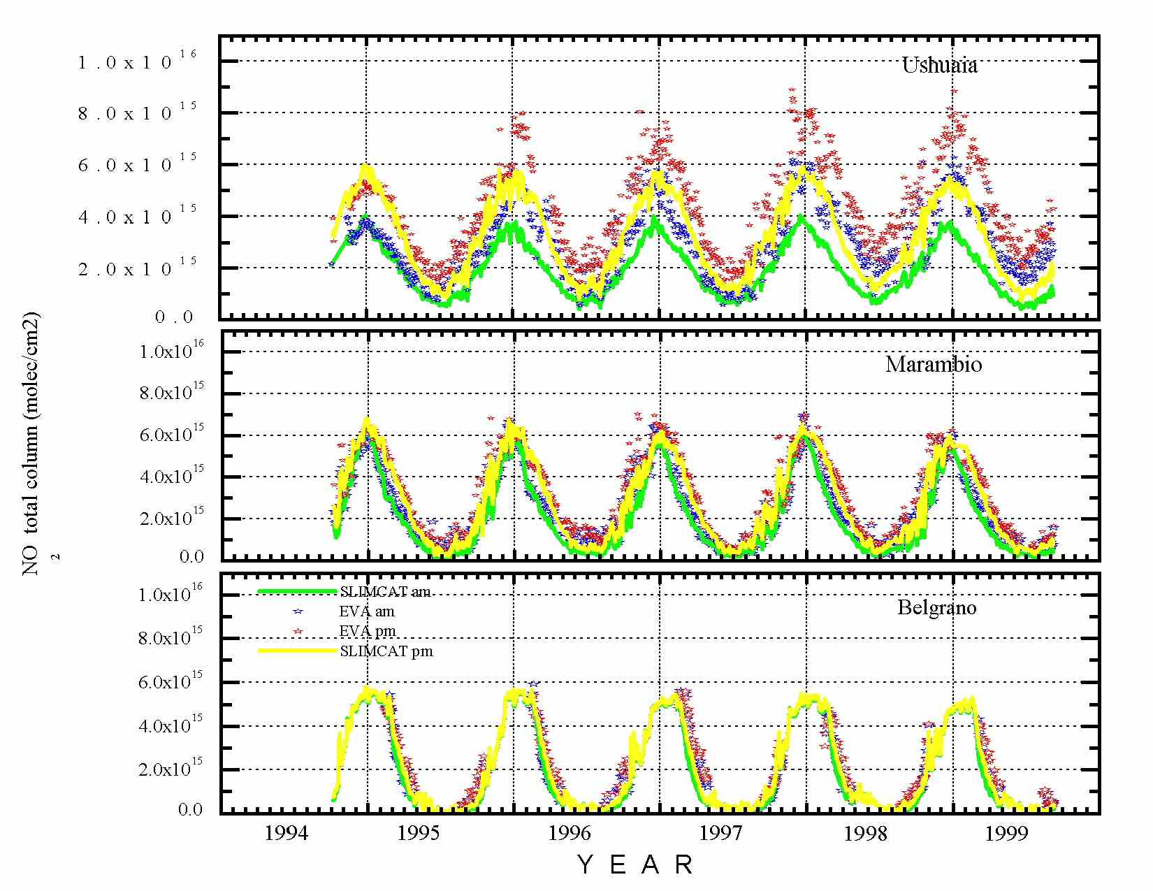
Figure 2. Evolution of the NO₂ column measured with the spectrometer and calculate with SLIMCAT modelling

The evolution of the NO₂ column with time as measured with the spectrometer is displayed in figure 2 (open stars). In solids lines the SLIMCAT modelling. The data are corrected from using room temperature cross sections to make comparable the results. The seasonal wave is well reproduced by the model but underestimates the NO₂ in Ushuaia (55ºS) during all seasons by 25-30%. Similar results were found at Northern Hemisphere mid latitudes (Chipperfield, 1999). Although part of the differences could be due to tropospheric NO₂ not included in the model, it seems that the model underestimates the NO₂ in the lower stratosphere. At higher latitudes the agreement is better. Marambio (64ºS) displays a seasonal wave of great amplitude with very low values in winter. A sharply maximum occurs around the summer solstice. General features are well reproduced by the model. Maxima and minima values are in close agreement. During both the equinoxes, however, the model remains below the data. Interannual variability is not high. Seasonal wave follows the hours of light per day and is modulated by the vortex position (PV) and by the temperature at 70 to 30 hPa.

The same situation is found in Belgrano (78ºS) although at this station no data are available for the solstices. It must be noted that during these periods the model computes the data at other sza than 90º (78º in summer, 102º in winter). The observed spring recovery is faster than that computed by the model.

A reduction in the summer maximum is observed in the last 3 years in both model and data over Marambio and in the model over Belgrano (no observational data available). These results are opposite of what has been found at mid latitudes in Southern Hemisphere (Liley et al. 2000). We have searched the lower stratospheric temperature to explore the origin of this reduction. From the NCEP data a negative trend is observed at lower level explored (70 hPa) above Belgrano (-0.83± 0.21 ºC/year) and Marambio (-0.43± 0.16 ºC/year) but not above Ushuaia. This negative trend takes place mainly in summer since winter minima remains without any significant change.

4.1.3. Column dependence on the amount of light.

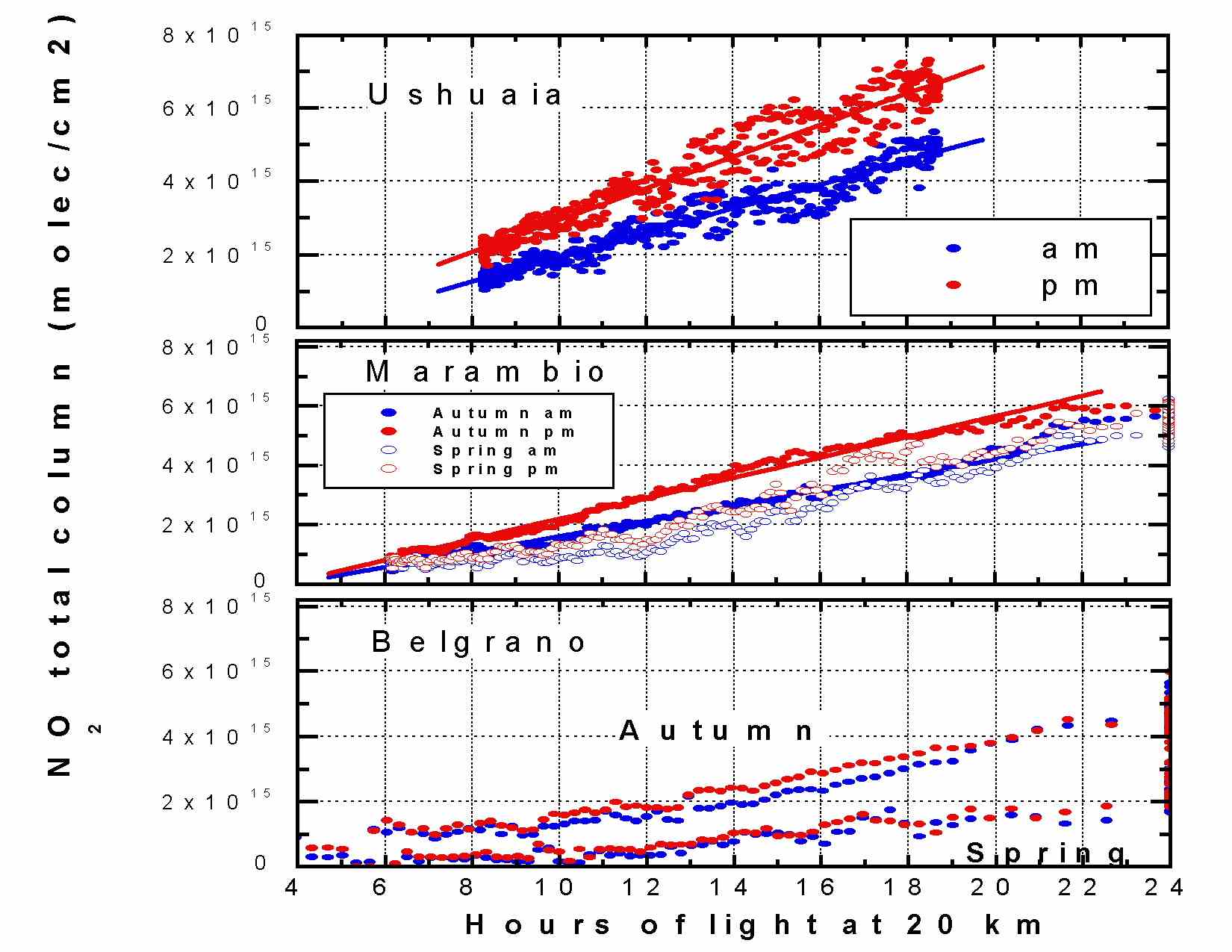
Figure 3. NO₂ total column against the hours of light available at 20 km

In order to make more comparable the data, NO₂ column for am and pm twilight have been plotted against the hours of light available at 20 km. In Ushuaia (55ºS) both datasets roughly follow linearity (figure 3, upper panel). The net daily production/destruction (average slope) is 4x10¹⁴ molec/cm² [3.7x10¹⁴ am and 4.3x10¹⁴ pm] per extra hour of light with a correlation coefficient of 0.96. By extrapolating, zero NO₂ is reached for 3-4 hours of light. In Marambio (64ºS) (figure 3, central panel) the correlation is even better (r² over 0.99) for autumn. As in the previous station, zero NO₂ is obtained for less than 3 hours of light. In spring strongly deviates from linearity, indicating other processes than pure photochemical and homogeneous chemistry. The observed lower values are due to the winter denitrification. For 12 hours of light, autumn to spring ratios reach a factor of 2 for am and still higher for pm values. The high day to day variability is related to the relative position of the station with respect of the vortex. Marambio is usually located at the edge of the vortex as can be seen by the PV charts and the total ozone fields from satellite (i.e. TOMS).

In Belgrano (78ºS) (figure 3, lower panel), the seasonal asymmetry between autumn and spring is significant. Autumn values reduce monotonically up to mid March. After this date, larger values of what could be expected by the available light are observed. Since the departure coincides in time with the start of the meridional transport season (NCEP reanalysis data, not shown), we attribute this feature to lower latitudes NOx transported toward the polar region before the vortex is formed. The amount (about 5x10¹⁴ molec/cm²) is too small to be observed in lower latitude stations. Spring values, either am and pm, remain within the instrumental detection limit up to the beginning of september.

4.1.4 PM-AM differences.

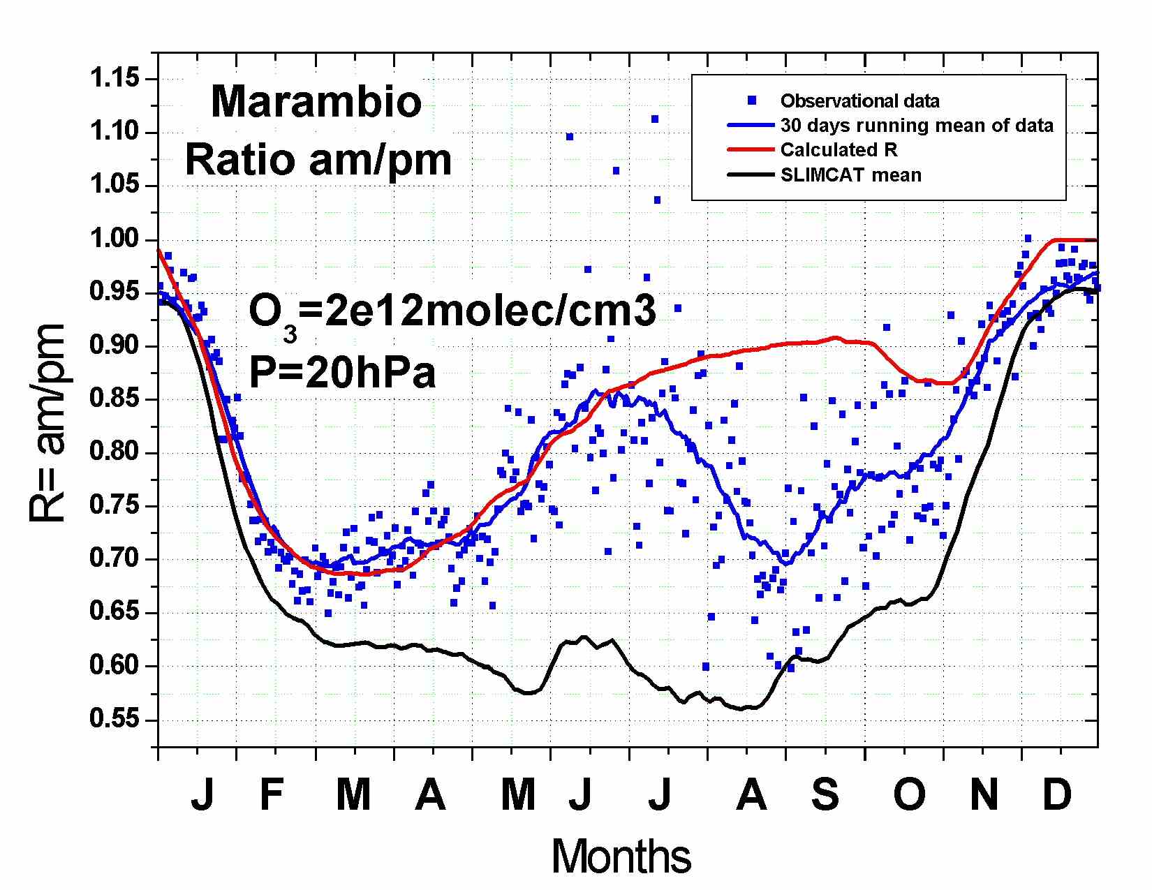
Figure 4. R calculate in Marambio

The diurnal increase of NO₂ at a given altitude and for a particular temperature is governed by the local concentration of ozone and the hours of available light as the increase takes place from N₂O₅ photodissociation created at night through reactions involving ozone (Keys and Gardiner 1991). The ratio (R) am/pm for a given altitude can be estimated from R=exp(-2k[O₃]t) (1) where k is the constant of the reaction of NO₂ with O₃, [O₃] is the ozone concentration and t is the duration of darkness.

R in Ushuaia is comprised between 0.6 and 0.8 all year around, with small seasonal dependence, since the decrease in temperature (k decrease) compensates the increase of hours of darkness. In Marambio, a biannual wave can be seen (figure 4, blue dots and line). Maxima are close to 1 during the solstices and minima of 0.7 during the equinoxes. The small diurnal variation during the solstices reflects the short distance in time between dawn and dusk. The increases in R from winter to spring can be reproduced considering that all ozone between 15 and 20 km has almost disappeared and no N₂O₅ can be formed. Consequently, the contribution to the diurnal variation (or R) in NO₂ comes from higher levels of 20 to 30 km. At these levels, the spring temperature is higher as heating inside the vortex is descending with time. The altitude that contributes to the bulk of NO₂ diurnal variation is changing with time. First ascending up to the end of September then descending again. A detailed study of the processes involved is in progress.

SLIMCAT yield higher R (black line) than observed and computed by (1). Seasonal variation is small. This higher values are, et least partly, related to the column underestimation in the model.

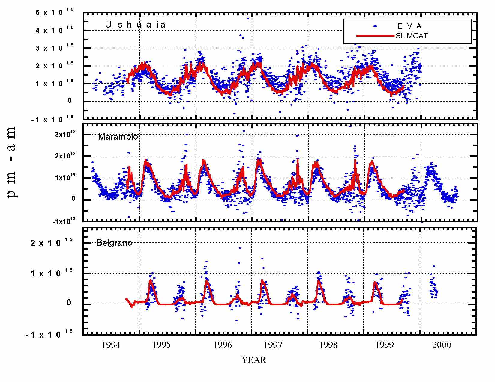
Figure 5. Diurnal variations are plotted as pm-am differences

In Belgrano there is a great scattering but values are not representative, particularly in spring, as the column is small. Occasionally, am values are higher than pm. This happens in periods with small photochemical changes (mid-summer, mid-winter) and it is attributed to transport processes.

A general comparison with SLIMCAT is shown in figure 5. Diurnal variations are plotted as pm-am differences. There is a good qualitative agreement but discrepancies can be shown. In Ushuaia the lower values in the model are related to the already mentioned underestimation in the column. Agreement is better in Marambio where also the best agreement in columns occurs. In mid-winter and early spring the model overestimated the observed data.

In Belgrano the agreement is good in autumn but at the end of the winter the model does not reproduce the negative values observed in the measurements. In this period of the year, the am-pm differences mostly result from horizontal transport due to homogeneities in NO₂ density inside the vortex, which cannot be resolved by the model.

4.2. O₃

4.2.1. Marambio. As Marambio is located at the edge of the Antarctic vortex, strong variability in ozone content takes place in scale of days during spring connected to the relative position of the vortex. As result, an annual average is misleading. We have therefore shown in figure 6 the O₃ evolution from the beginning of measurements (1994-2000). TOMS data and SLIMCAT are also shown. The potential vorticity (PV) at 475K is displayed to indicate the relative position of the vortex. O₃ values in days with PV below ­45 PVU can be unequivocally considered as belonging to in-vortex air. In general, Marambio is during spring inside the vortex. However, there are episodes when the vortex elongates with axis in direction 0º-180º in longitude and mid-latitude air reaches the station resulting in ozone variations of up to 275 DU in ten days (Yela et al 1998). Those short episodes are well reproduced by SLIMCAT. The highest discrepancy between model and data takes place in winter when no TOMS neither ground based direct sun instruments are available. SLIMCAT show a continuous decrease in ozone of 15 DU/month from the maximum close to the summer solstice. Data, however, present an increase in winter. The same situation occurs in Belgrano, as will be described later.

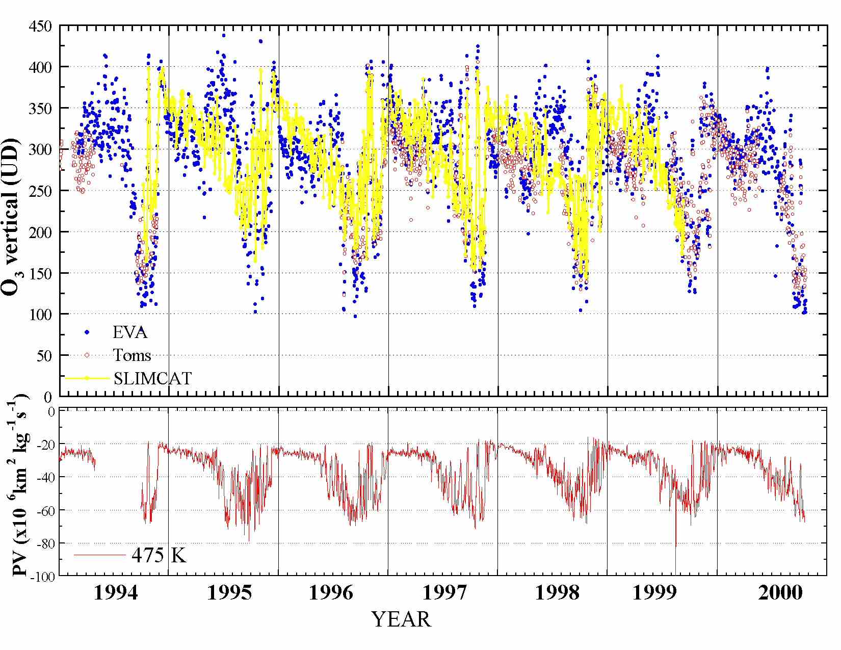
Figure 6. O₃ evolution over Marambio with PV values at 475 K

4.2.2. Belgrano.

As Belgrano is usually inside the vortex in spring, the interannual variability is small, and seasonal characteristics can be explored by using accumulated data (figure 7). SLIMCAT results are available for all the year round. TOMS gap during the polar night extends from April to September. Spectroscopic data are available in two periods; from late summer to mid autumn and from late winter to mid spring. As for Marambio, SLIMCAT overestimates the ozone in summer. In autumn all datasets agree. Discrepancy with the model is highest in August. Spectroscopic data seems to overestimate the amount of ozone when the sun is too low (below sza of 91º at end of April and beginning of August). However, TOMS data in September appear to provide a confirmation that in any case SLIMCAT is underestimating the ozone amount in that period. This belief is supported by the integrated data from ozonesondes above the station. The behaviour is found to be the same for all years. The model shows an almost linear decrease in the column starting at the end of the summer of about 25 DU/month. By the beginning of August it is already at 225 DU in average, that is 32% lower than in January-February.

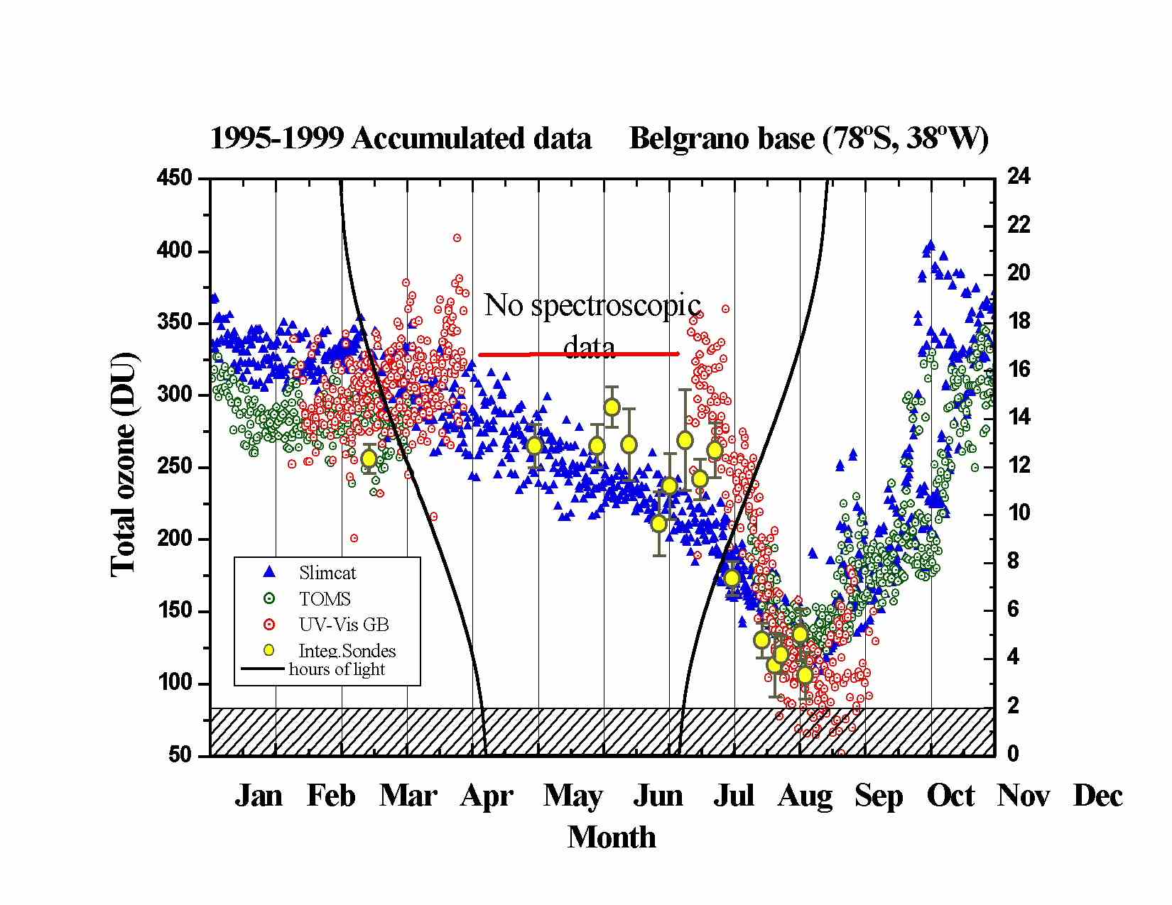
Figure 7. Accumulated O₃ data in Belgrano.

The model lower values result from contributions from lower latitudes due to the size of the grid (7.5ºx7.5º), too coarse for polar regions. As Roscoe et al. [1997] have shown, depletion start in winter at the illuminated areas, that is in a belt around 60-70º, extending to the pole as time proceed.